Selecting Grains

A grain2d variable is a list of grains. Selecting grains means indexing that list by position, phase, property, spatial coordinates, or mean orientation. Every selection is another grain list, so selections can be applied one after another.

This page assumes that you have reconstructed grains as described in Grain Reconstruction. It also assumes that you can draw them as in Plotting Grains.

import matplotlib.pyplot as plt
import numpy as np

from mtex import *

# load sample EBSD data set
plottingConvention.default('y↑→x')
ebsd = mtexdata('forsterite')

# restrict it to a subregion of interest
ebsd = ebsd[ebsd.inpolygon(np.array([5, 2, 10, 5]) * 1e3)]

# reconstruct grains; their ids are stored with the measurements
grains = calcGrains(ebsd, angle=5 * degree, minPixel=5, alpha=6)

# smooth the boundaries
grains = smoothBoundary(grains, 5)

# plot forsterite by orientation
plot(ebsd['Fo'], ebsd['Fo'].orientations, ipfDirection=zvector)

# plot the other two phases in grey
hold(True)
plot(ebsd['En'], faceColor='lightgray')
plot(ebsd['Di'], faceColor='darkgray')
plot(grains.boundary, lineWidth=2)
hold(False)

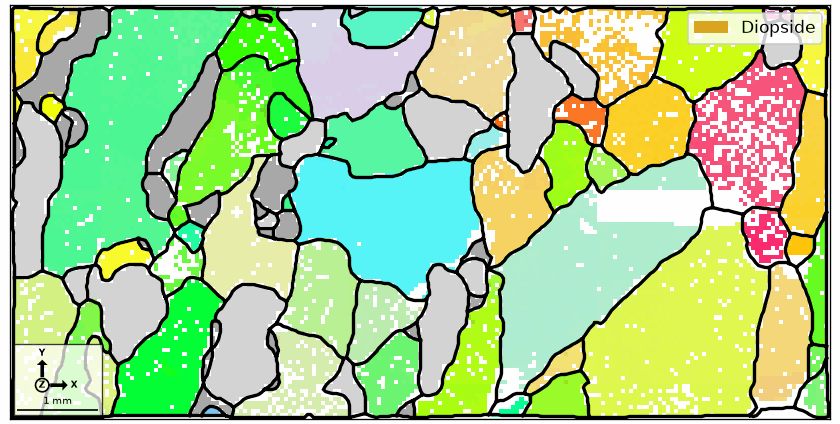
The black network outlines every reconstructed grain. The forsterite measurements retain their orientation colours, while the two minor phases are grey so that later highlights remain easy to see.

By mouse

In MATLAB, selectInteractive installs a mouse callback on the current figure. A click selects one grain, and additional clicks extend the selection, and the global variable indSelected stores the selected positions in the current grain list. There is no mouse selection in this port; the same result comes from the grain at a known coordinate, whose position in the list id2ind looks up from its id.

indSelected = grains.id2ind(grains(9000, 3500).id)

mouseGrains = grains[indSelected]
mouseGrains

grain2d (y↑→x)
  size: 1
  Phase  Grains          Mineral     Color         Symmetry  Crystal reference frame
  1      1 (323 pixels)  Forsterite  LightSkyBlue  mmm       Forsterite
  boundary segments: 87, inner: 0, triple points: 6
        Id   Phase  Pixels        meanRotation         GOS
        26       1     323     (131°,64°,250°)     0.00795

hold(True)
plot(mouseGrains.boundary, lineWidth=4, lineColor='gold')
hold(False)

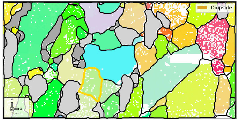
The gold outline marks the selected grain. If several grains had been clicked, every selected outline would be gold and mouseGrains would contain all of them.

By position

The expression grains(x, y) returns the grain containing the point (x, y) in map coordinates. It needs neither a figure nor a mouse click.

x = 12000
y = 4000

hold(True)
plot(grains(x, y).boundary, lineWidth=4, lineColor='blue')
plt.plot(x, y, marker='s', markerfacecolor='k', markersize=10, markeredgecolor='w', label='A')
hold(False)

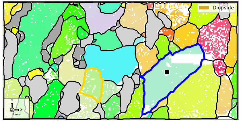
Marker A lies inside the thick blue outline. The coordinate is used for the lookup; its location in the current axes does not affect the result.

By phase

A grain is phase-homogeneous. A mineral name therefore selects every grain of that phase, and the displayed summary reports what came back.

forsteriteGrains = grains['forsterite']
forsteriteGrains

grain2d (y↑→x)
  size: 61
  Phase  Grains             Mineral     Color         Symmetry  Crystal reference frame
  1      61 (14010 pixels)  Forsterite  LightSkyBlue  mmm       Forsterite
  boundary segments: 2819, inner: 12, triple points: 133

The mineral name is the readable form of a condition on phase. This property stores one imported phase number per grain.

firstFivePhase = grains[0:5].phase
firstFivePhase

array([1, 1, 1, 1, 3])

By a property

A grain property has one value per grain. NumPy operations on arrays can therefore build indices from any such property. We begin with area.

grainArea = grains.area

plot(grains, grainArea)

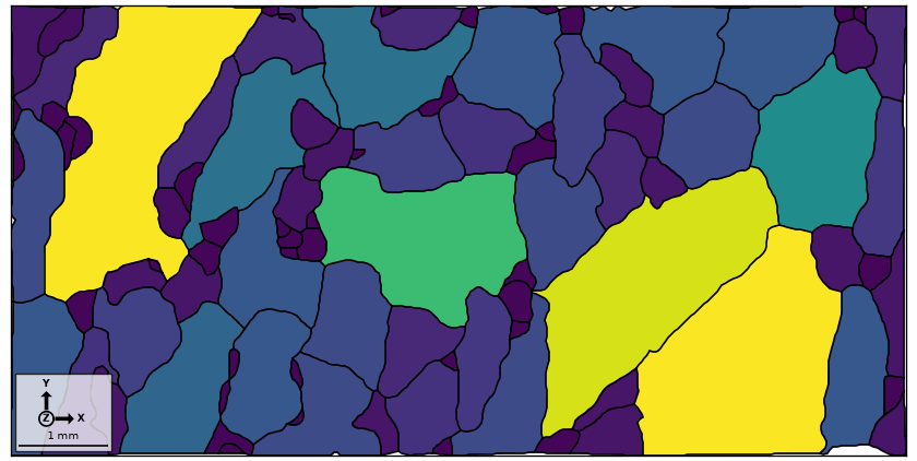
Large grains are bright and small grains are dark. This map shows where the extremes lie before any threshold is imposed.

np.argmax returns the position of the largest value in the list. That position is an index, not a persistent grain ID.

maxIndex = np.argmax(grainArea)
maxArea = grainArea[maxIndex]
maxArea

4.0983e+06

maxIndex

38

hold(True)
plot(grains[maxIndex].boundary, lineColor='red', lineWidth=4)
hold(False)

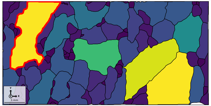
The red outline encloses the brightest grain in the area map. Sorting generalises this selection from one grain to the largest few.

sortedIndex = np.argsort(-grainArea)

# select the second to fifth largest grains
hold(True)
plot(grains[sortedIndex[1:5]].boundary, lineColor='orange', lineWidth=4)
hold(False)

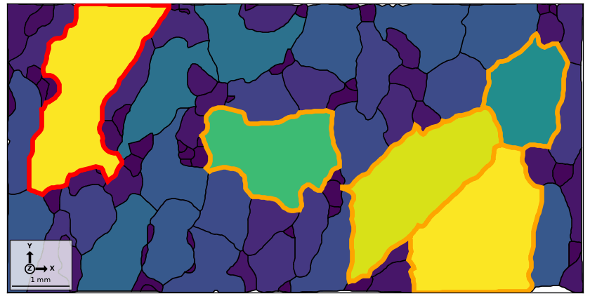
The orange outlines mark ranks two through five. The largest grain remains identifiable by its red outline from the preceding selection.

By a condition

A logical array with one value per grain can index the list directly. Here it selects every grain at least one quarter the size of the largest.

condition = grainArea > maxArea / 4

hold(True)
plot(grains[condition].boundary, lineColor='yellow', lineWidth=4)
hold(False)

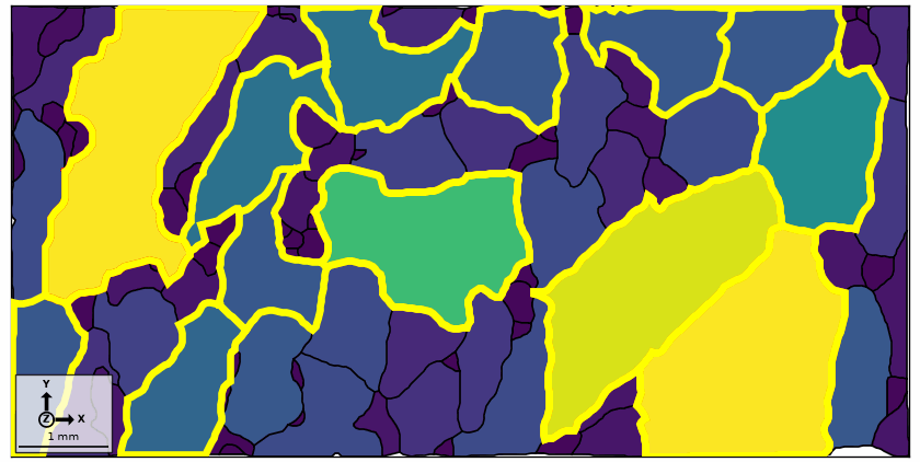
The yellow outlines include more grains than the fixed rank selection. Their membership follows an area threshold rather than a chosen count.

Conditions may be combined. The next selection requires a perimeter above 6000 map units and at least 600 measurements. The pixel-count condition excludes grains too small for their outline to support a useful shape interpretation.

condition = (grains.perimeter > 6000) & (grains.numPixel >= 600)

selectedGrains = grains[condition]
selectedGrains

grain2d (y↑→x)
  size: 4
  Phase  Grains           Mineral     Color         Symmetry  Crystal reference frame
  1      4 (5248 pixels)  Forsterite  LightSkyBlue  mmm       Forsterite
  boundary segments: 736, inner: 0, triple points: 43
        Id   Phase  Pixels        meanRotation         GOS
        14       1    1448    (166°,127°,259°)      0.0135
        19       1    1208     (153°,68°,237°)     0.00808
        34       1    1047      (89°,99°,224°)     0.00769
        39       1    1545     (167°,81°,251°)       0.013

plot(selectedGrains)

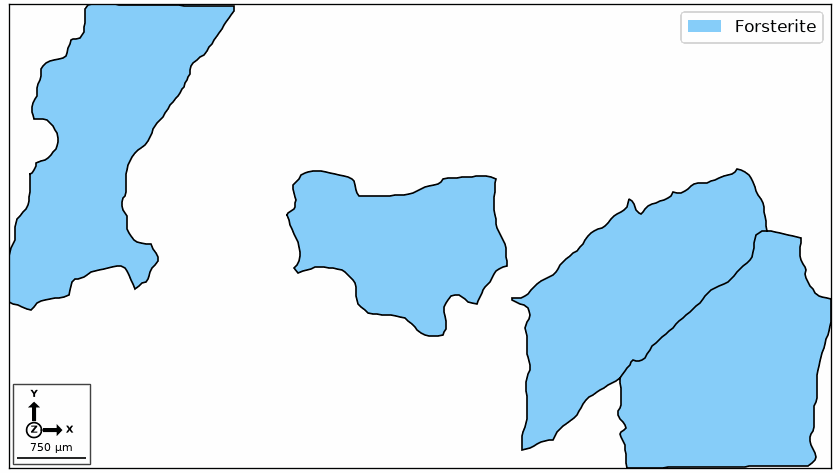
Only the grains satisfying both conditions remain in the plot. Empty spaces belong to grains excluded by at least one condition.

By orientation

findByOrientation selects grains whose mean orientation lies within a specified angle of a reference orientation. It accounts for crystal symmetry, so equivalent descriptions of the same lattice orientation are treated as the same orientation.

We use the first gold grain from above as the reference and a threshold of 20 degrees.

referenceGrain = mouseGrains[0]
similarGrains = grains.findByOrientation(referenceGrain.meanOrientation, 20 * degree)
similarGrains

grain2d (y↑→x)
  size: 3
  Phase  Grains          Mineral     Color         Symmetry  Crystal reference frame
  1      3 (523 pixels)  Forsterite  LightSkyBlue  mmm       Forsterite
  boundary segments: 164, inner: 0, triple points: 13
        Id   Phase  Pixels        meanRotation         GOS
        25       1     181     (131°,64°,245°)     0.00698
        26       1     323     (131°,64°,250°)     0.00795
        58       1      19     (144°,74°,250°)      0.0104

plot(ebsd['Fo'], ebsd['Fo'].orientations, ipfDirection=zvector)
hold(True)
plot(grains.boundary, lineWidth=2)
plot(similarGrains.boundary, lineWidth=4, lineColor='gold')
hold(False)

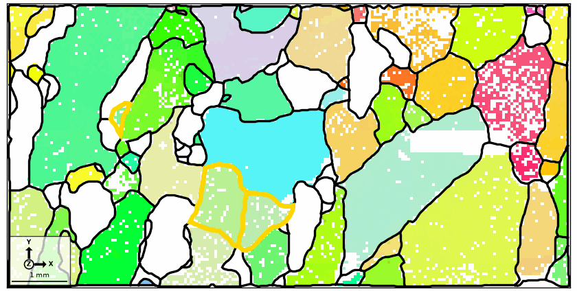
Three grains are selected, and two share a boundary. Neighbours with mean orientations this close deserve a second look. The reconstruction may have split one grain, or the grains may have belonged together before another process separated them. Merging Grains develops this question.

List position and grain ID

A list position answers “which entry of this variable?” A grain ID answers “which reconstructed grain?” They are initially often equal, but a subset keeps the original IDs while its positions start again at zero.

plot(grains)
largeGrains = grains[grains.numPixel > 50]
text(largeGrains, largeGrains.id)

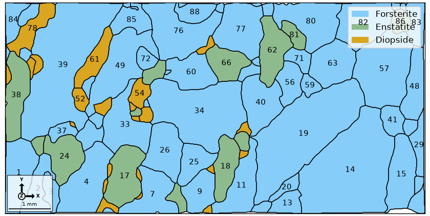
The labels are persistent grain IDs. They are not the positions of the labelled grains in largeGrains.

listPosition = 0
grainId = largeGrains.id[listPosition]
print(f'list position {listPosition} has grain ID {grainId}')

grainByPosition = largeGrains[listPosition]
grainById = largeGrains['id', grainId]
sameGrain = grainByPosition.id == grainById.id
sameGrain

list position 0 has grain ID 1
array([ True])

largeGrains[0] selects by position. The form largeGrains['id', grainId] searches the stored IDs. The printed logical value confirms that both expressions identify the same grain here.

From grains back to measurements

Every grain selection can be converted to the measurements it contains. This requires the grainId property that calcGrains wrote into the map.

measurementsByGrain = ebsd[grainById]
measurementsByGrain

EBSD (y↑→x)
  size: 405
  Phase  Orientations  Mineral     Color         Symmetry  Crystal reference frame
  1      405 (100%)    Forsterite  LightSkyBlue  mmm       Forsterite
  properties    : bands, bc, bs, error, grainId, mad
  scan unit     : um
  X × Y         : [5000 → 5750] × [2000 → 3750]
  square lattice: spacing 50

measurementsById = ebsd[ebsd.grainId == grainId]
sameMeasurements = np.array_equal(measurementsByGrain.id, measurementsById.id)
sameMeasurements

True

The first command displays the selected measurements. The printed logical value confirms that selecting by the grain object and matching the stored ebsd.grainId return the same subset.

Applied to the largest grain, this relationship reveals the orientations measured inside one reconstructed grain.

largestGrain = grains[maxIndex]
largestGrainEbsd = ebsd[largestGrain]

plot(largestGrainEbsd, largestGrainEbsd.orientations, ipfDirection=zvector)
hold(True)
plot(largestGrain.boundary, lineWidth=2)
hold(False)

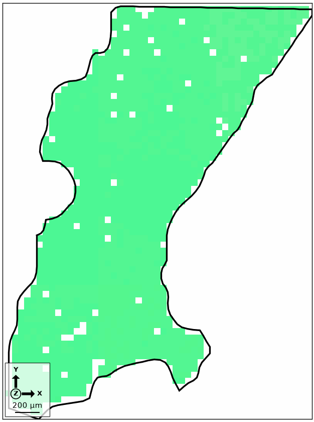
The colours inside the black outline come from the individual measurements, not from one grain mean. On this grain the spread is small, under two and a half degrees, so the fill reads as a single shade and the unindexed white pixels are what stands out.

A spread this size has to be measured rather than looked for. The mean and spread of the distribution are the subject of Grain Orientation Parameters.

Grains at the edge of the map

A grain touching the map edge continues outside the measured region. Its observed area and shape describe only the measured piece. Remove such grains before calculating per-grain size or shape statistics with isBoundary.

interiorGrains = grains[~grains.isBoundary]
plot(interiorGrains)

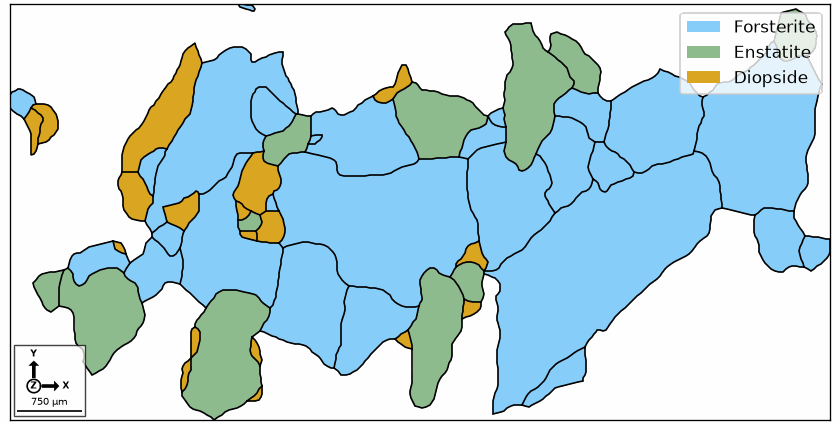
The white band around the plot is occupied by the omitted edge grains. This exclusion is appropriate for comparing complete observed shapes. A standardised average grain-size measurement may prescribe a different boundary-counting rule, so follow the selected standard when reporting one.

The boundary network shows what isBoundary tests. Each grain boundary segment stores the IDs of the two grains it separates. A segment at the map edge has no grain on one side, so the corresponding ID is zero.

# find segments with zero on one side
isOuterBoundary = np.any(grains.boundary.grainId == 0, axis=1)

plot(grains)
hold(True)
plot(grains.boundary[isOuterBoundary], lineColor='red', lineWidth=2)
hold(False)

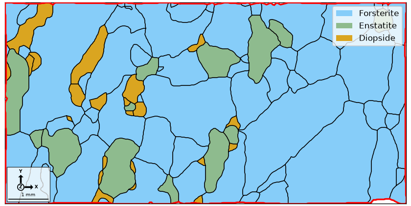
The red segments form the outer rim of the measured region. Their nonzero IDs identify exactly the grains removed above.

boundaryGrainId = grains.boundary[isOuterBoundary].grainId
boundaryGrainId = np.unique(boundaryGrainId[boundaryGrainId != 0])

plot(grains['id', boundaryGrainId])

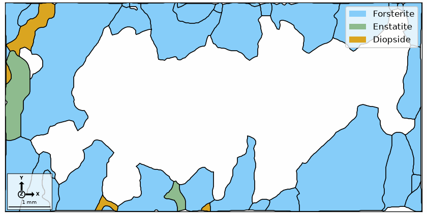
Only the edge grains remain. The explicit 'id' lookup is required because the values came from grainBoundary.grainId rather than from list positions.

Next

Shape Parameters defines the area, perimeter, and other geometric properties used to build selections. The ellipse, convex hull, and projection pages that follow it provide further shape measures. Grain Orientation Parameters develops selections based on the orientation distribution inside each grain.

Grain selections also lead back to the boundary network. Selecting Grain Boundaries selects its segments, and Merging Grains uses selected boundaries to join grains.

Further reading

• F. Bachmann, R. Hielscher, and H. Schaeben, “Grain detection from 2d and 3d EBSD data - Specification of the MTEX algorithm”, Ultramicroscopy 111 (2011), 1720-1733, doi:10.1016/j.ultramic.2011.08.002. This paper derives the Voronoi-cell grain model whose IDs connect the grain list to the EBSD measurements.

• ASTM E2627-13(2019), Standard Practice for Determining Average Grain Size Using Electron Backscatter Diffraction (EBSD) in Fully Recrystallized Polycrystalline Materials.

• ISO 13067:2020, Microbeam analysis - Electron backscatter diffraction - Measurement of average grain size. It distinguishes measurements on a two-dimensional section from inferences about three-dimensional grain size.

Technical details

List positions count from zero, as Python indexes, while grain ids count from one as MATLAB’s do. selectInteractive has no counterpart; a marker on the map is matplotlib’s plt.plot at the map coordinates, which are the screen coordinates under y↑→x.

@article{bachmann2010mtex,
  author  = {F. Bachmann and R. Hielscher and H. Schaeben},
  title   = {Texture Analysis with MTEX - Free and Open Source Software Toolbox},
  journal = {Solid State Phenomena},
  volume  = {160},
  pages   = {63-68},
  year    = {2010},
  doi     = {10.4028/www.scientific.net/SSP.160.63},
  url     = {https://doi.org/10.4028/www.scientific.net/SSP.160.63}
}