
A reconstructed grain is represented by the orientations measured at all of its EBSD points. Grain orientation parameters reduce that orientation cloud to three questions: where is its centre, how wide is it, and does it have a preferred direction of spread?
meanOrientation |
mean orientation | GOS |
grain orientation spread |
GAM |
grain average misorientation | GAX |
grain average misorientation axis |
The last label is used inconsistently. This page does not average misorientation axes to obtain GAX. It fits a fibre to the orientation cloud and calls the result a dispersion axis.
The example is a deformed ferrite map. It assumes familiarity with grain reconstruction and misorientations. See Selecting Grains for the relation between a grain and its EBSD points.
import numpy as np
from mtex import *
# use the map frame shown throughout this example
plottingConvention.default('y↓→x')

# import the data
ebsd = mtexdata('ferrite')

# reconstruct grains; one grain id per measurement is stored with the map
grains = calcGrains(ebsd, angle=7.5 * degree, minPixel=5)
ebsd = ebsd.projectIntoFundamentalRegion()

# smooth only the outlines used in the figures, and keep the indexed grains
grains = smoothBoundary(grains, 5)
grains = grains['indexed']

# use one colour key for the measurement and grain-mean maps
ipfKey = ipfColorKey(ebsd.CS)
ebsdColor = ipfKey.orientation2color(ebsd.orientations)

# plot the measured orientations and reconstructed grain boundaries
plot(ebsd, ebsdColor)
hold(True)
plot(grains.boundary, lineWidth=2)
hold(False)
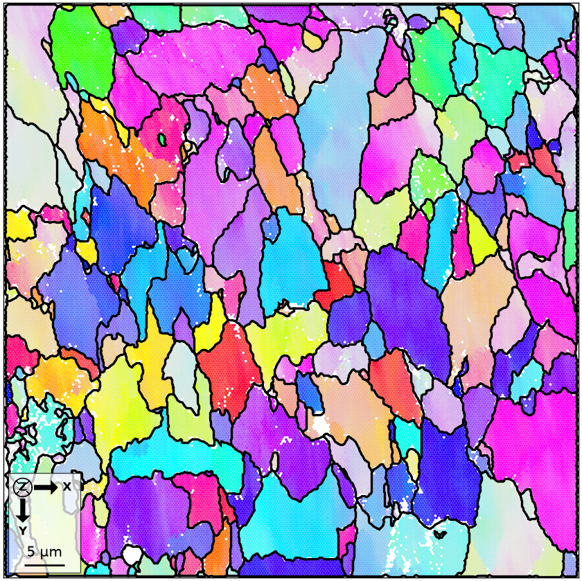
The colour changes inside the black outlines are the intragranular orientation variations measured below. Boundary smoothing changes the drawn outlines, but not which measurement belongs to which grain.
The mean orientation
Select one grain by its map coordinates. Indexing the EBSD map with that grain follows
ebsd.grainId and returns all measurements assigned to it.
# select a grain by x and y coordinates
grainSel = grains(42, 17)

# display all EBSD orientations within the grain
ori = ebsd[grainSel].orientations
ori
orientation (Ferrite → y↓→x)
  size: 1964
  Bunge Euler angles in degree
  phi1   Phi  phi2
   320  40.4  32.1
   321  40.2  31.1
   321  40.8  31.2
   321  39.4  30.4
   320  38.1  28.4
     ⋮     ⋮     ⋮
   328  39.5  28.6
   327  40.2    31
   328    40  30.5
   328  39.8  29.5
   328  39.8  28.9
The summary reports how many orientations represent this grain. Their mean is the
symmetry-aware centre of the cloud, not an arithmetic mean of Euler angles.
calcGrains has already stored this result as grains.meanOrientation. There is no
reason to compute it again.
meanColor = ipfKey.orientation2color(grains.meanOrientation)
plot(grains, meanColor, micronbar=False)
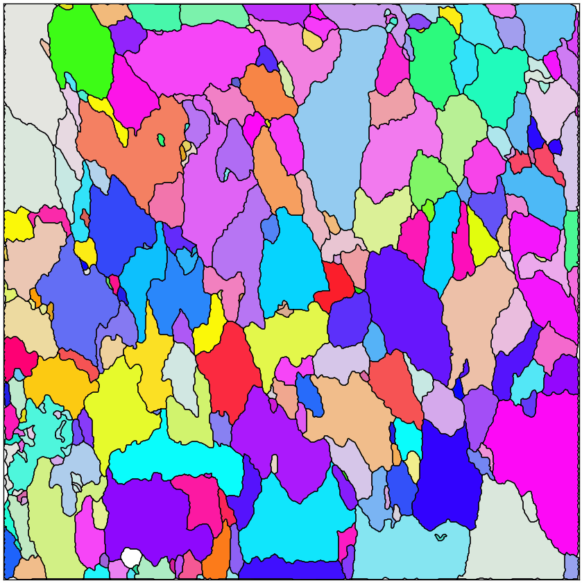
The map assigns one mean orientation colour to each grain. It therefore removes the within-grain colour gradients visible in the first map while preserving the orientation contrast between grains.
Deviation from the mean
With one reference orientation per grain, every measurement can be described by how far it departs from that reference. The resulting misorientation is the grain reference orientation deviation, GROD.
mis2meanSelected = grainSel.meanOrientation.inv() * ori
calcGROD performs the same calculation for the whole map and uses the appropriate mean
orientation for each grain ID.
mis2mean = calcGROD(ebsd, grains)
Grain orientation spread
A misorientation has an angle and an axis. Averaging only the GROD angle over a grain
gives the grain orientation spread, GOS. grainMean averages any per-measurement
quantity over grains.
# average the GROD angles for each grain
GOS = grainMean(ebsd, mis2mean.angle(), grains)

# plot the result in degrees
plot(grains, GOS / degree, micronbar=False)
mtexColorbar(title='GOS in degree')
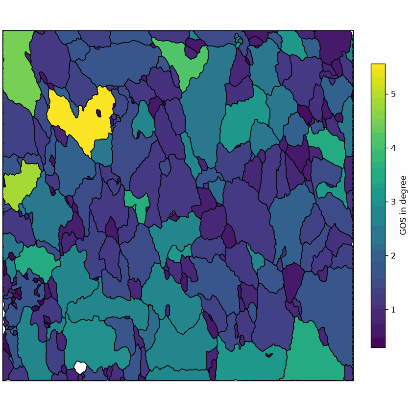
Grains that are internally uniform are dark. Grains with a larger orientation gradient stand out, but GOS alone does not reveal the shape or direction of that gradient.
The same value is available as grains.GOS because calcGrains computed it from the
orientations used for reconstruction. If the orientations are subsequently denoised or
otherwise changed, recompute GROD and GOS instead of treating the stored value as
updated.
grainMean accepts a function as a further argument. Using np.max gives the largest
deviation in each grain rather than the average. A median, a quantile, or another
statistic can be used in the same way.
# compute the maximum GROD angle for each grain
MGOS = grainMean(ebsd, mis2mean.angle(), grains, np.max)

# plot it
plot(grains, MGOS / degree, micronbar=False)
mtexColorbar(title='maximum GROD in degree')
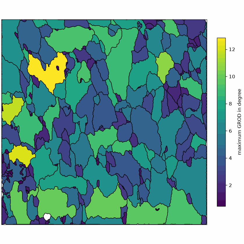
The maximum map emphasizes isolated peaks and sharp internal changes. The GOS map is less sensitive to one extreme measurement because it averages over the whole grain.
Grain average misorientation
GOS compares every measurement with the mean of its grain. It therefore grows with the total orientation change across a large grain, even when the change is gentle.
The grain average misorientation, GAM, asks a local question instead. It is the
kernel average misorientation averaged over each grain. The default KAM
compares first-order neighbours, applies no angle threshold, and does not cross
reconstructed grain boundaries when ebsd.grainId is present.
kam = ebsd.KAM()
gam = grainMean(ebsd, kam, grains)

plot(grains, gam / degree, micronbar=False)
mtexColorbar(title='GAM in degree')
setColorRange([0, 3])
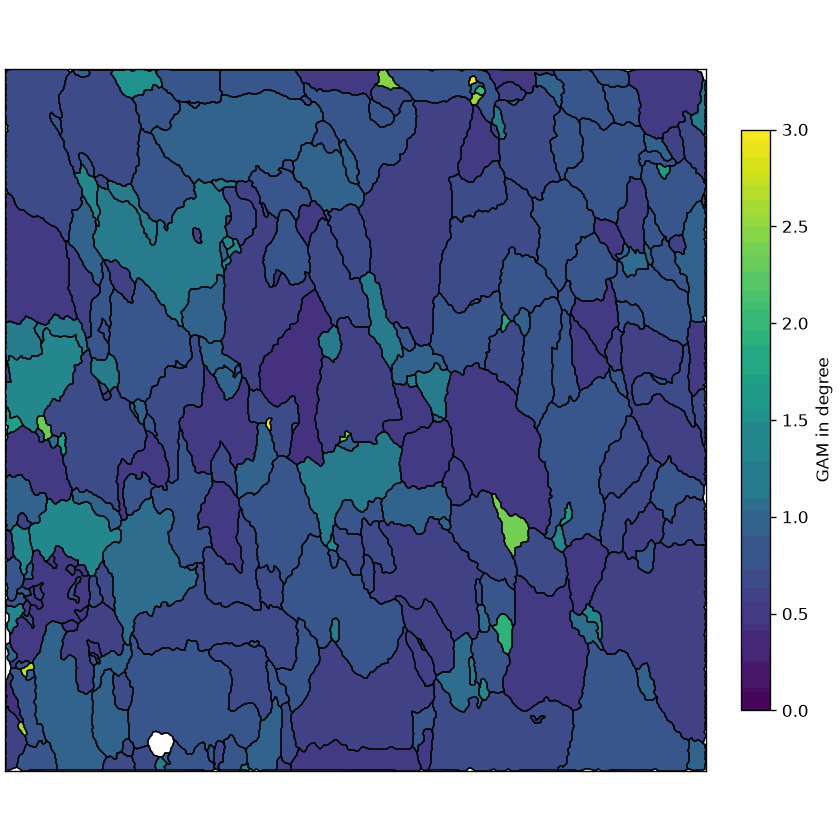
The GOS and GAM maps do not agree, and they are not meant to. GOS measures the total orientation change across a grain, whereas GAM measures the mean steepness of the local changes. A grain bent smoothly from one side to the other can have high GOS and low GAM. A subgrain boundary can instead produce high GAM. The two measures are regularly confused in the literature.
Neither quantity is a direct strain or dislocation-density measurement. Segmentation, grain size, scan step, angular precision, denoising, and the KAM neighbourhood all affect the result. Report those choices whenever GOS or GAM is compared between maps.
The crystal dispersion axis
Slip on one dominant system can spread the orientations of a grain along a curve rather than equally in every direction. Such a curve is an orientation fibre. Its axis may constrain the slip system that produced the orientation gradient.
fibre.fit finds the fibre that best fits a list of orientations. It always returns a
fibre, even for a round cloud, so the fit must be checked before its axis is
interpreted.
# visualize the selected grain orientations in a pole figure
h = Miller(1, 0, 0, ebsd.CS)
plotPF(ori, h, markerSize=2, all=True)

# fit a fibre to those orientations
f, lam, fit = fibre.fit(ori, 'local', diagnostics=True)

# add the fibre to the pole figure
hold(True)
plotPF(f.symmetrise(), h, lineColor='orange', lineWidth=2)
hold(False)
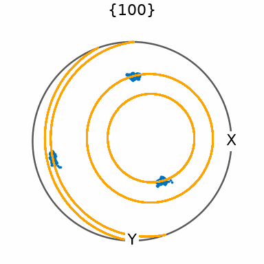
The orientations lie in short streaks rather than round blobs, and the orange fibre
follows them. The fitted axis is f.r in the specimen frame and f.h in the crystal
frame.
axisSpecimen = f.r
axisSpecimen
vector3d (y↓→x)
       x       y      z
  -0.282  0.0471  0.958
axisCrystal = f.h
axisCrystal
vector3d (Ferrite)
       u       v       w
  0.0182  0.2054  0.2808
Rotation about an axis leaves that axis itself fixed. The crystal direction f.h should
therefore scatter less than the other directions in the pole figure.
hold(True)
plot(ori * f.h, markerSize=2, all=True, markerFaceColor='k', antipodal=True)
hold(False)
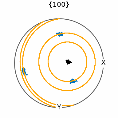
The black points form a compact cluster where the other poles form streaks. This is a direct visual check on the fitted crystal axis.
The second output of fibre.fit contains four eigenvalues of the orientation tensor in
ascending order. The largest describes the overall concentration. The second largest,
lam[2], describes spread along the fitted fibre. The two smallest describe scatter
away from it; lam[1] is the larger of those two. The third output is the mean angular
distance from the orientations to the fibre.
lam
array([0.0001, 0.0001, 0.0004, 0.9994])
fitDegrees = fit / degree
fitDegrees
1.2233
Fitting every sufficiently large grain
A separate fibre must be fitted to each grain. Very small grains contain too few orientations to define the shape of an orientation cloud, so the example keeps grains with more than 50 measurements.
grainsLarge = grains[grains.isIndexed & (grains.numPixel > 50)]
nLarge = len(grainsLarge)
lam = np.full((nLarge, 4), np.nan)
fit = np.full(nLarge, np.nan)
GAX_C = np.full((nLarge, 3), np.nan)
GAX_S = np.full((nLarge, 3), np.nan)

# fit one fibre per grain and store its axes in both frames
for k in range(nLarge):

  f, lam[k], fit[k] = fibre.fit(ebsd[grainsLarge[k]].orientations, 'local', diagnostics=True)
  GAX_C[k] = f.h.data.reshape(3)
  GAX_S[k] = f.r.data.reshape(3)

GAX_C = Miller(vector3d(GAX_C), ebsd.CS)
GAX_S = vector3d(GAX_S, frame=ebsd.frame)
The ratio lam[:, 2] / lam[:, 1] compares spread along the fibre with scatter away from
it. A ratio near 1 describes a blob rather than a line. The threshold 3 used below is a
screening choice, not a universal material constant.
linearity = lam[:, 2] / lam[:, 1]
isFibre = linearity > 3

corrFitLambda2 = np.corrcoef(fit, lam[:, 1])[0, 1]
corrFitLambda3 = np.corrcoef(fit, lam[:, 2])[0, 1]

print(f'large grains: {nLarge}, accepted axes: {np.count_nonzero(isFibre)}, corr(fit, lambda2): {corrFitLambda2:.5f}, '
      f'corr(fit, lambda3): {corrFitLambda3:.5f}, fit from {np.min(fit) / degree:.5f} to {np.max(fit) / degree:.4f} degrees')
large grains: 161, accepted axes: 103, corr(fit, lambda2): 0.92299, corr(fit, lambda3): 0.63697, fit from 0.25359 to 2.2591 degrees
The table makes the screening reproducible. Of the 161 large grains, 103 pass the ratio
threshold. Fit and lam[:, 1] correlate at 0.92, whereas fit and lam[:, 2] correlate
at 0.61. The fit angles range from 0.25 to 2.18 degrees.
This is expected because fit measures scatter away from the fibre. A grain worth
reading a dispersion axis from has large lam[:, 2], small lam[:, 1], and therefore a
large ratio.
newMtexFigure(layout=[1, 3], figSize=(14, 4))
plot(grainsLarge, lam[:, 2], micronbar=False)
mtexTitle('$\\lambda_3$')

nextAxis()
plot(grainsLarge, lam[:, 1], micronbar=False)
mtexTitle('$\\lambda_2$')

nextAxis()
plot(grainsLarge, fit / degree, micronbar=False)
mtexTitle('fit in degree')
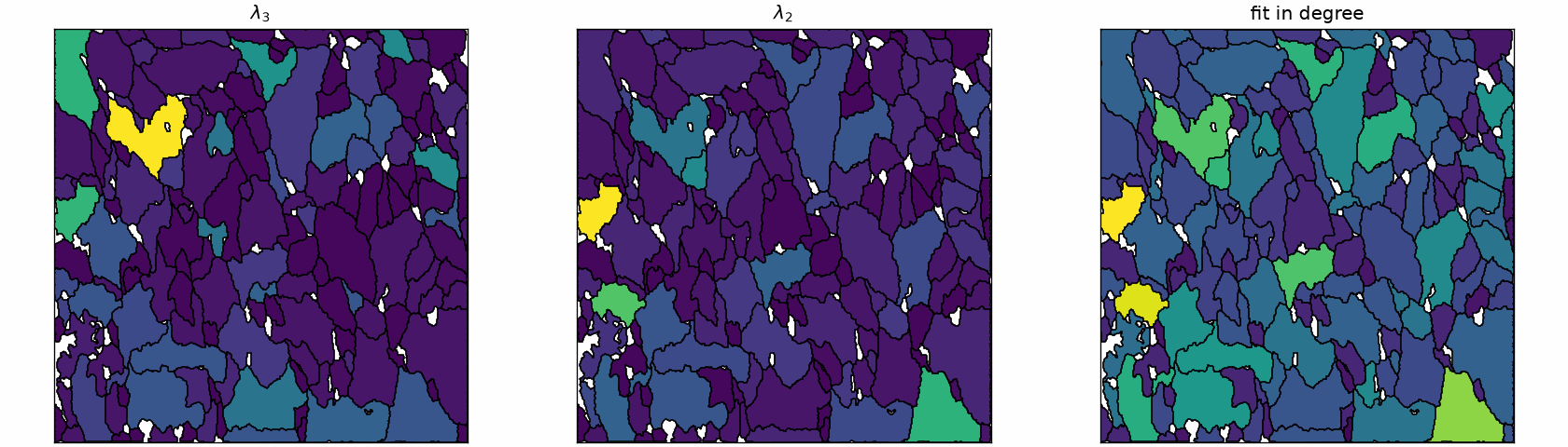
The lam[:, 2] map shows where orientation clouds extend along a fibre. The lam[:, 1]
and fit maps instead highlight scatter away from that fibre. Their visual similarity
agrees with the correlations in the table.
Axes in crystal coordinates
The fitted axes are crystal directions. An HSVDirectionKey colours those directions,
and it needs antipodal because an axis and its negative are the same axis.
# define the colour key
cKey = HSVDirectionKey(ebsd.CS, antipodal=True)

# plot the key and the accepted dispersion axes
plot(cKey)
hold(True)
plot(projectIntoFundamentalRegion(GAX_C[isFibre], antipodal=True), markerFaceColor='black')
hold(False)
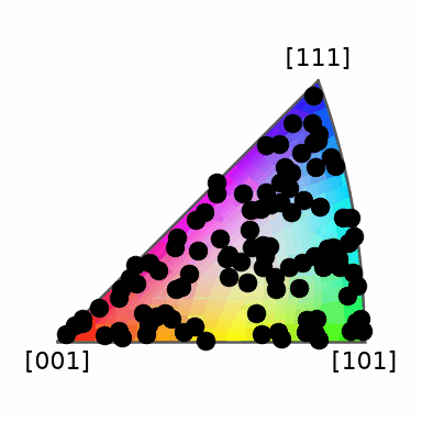
The black dots show which crystal directions occur as credible axes. A cluster would point to a preferred crystal direction and could constrain a common slip mechanism. The colours below show where grains with similar axes lie in the map.
# compute colours from the accepted crystal axes
color = cKey.direction2color(GAX_C[isFibre])

# plot the corresponding grains
plot(grainsLarge[isFibre], color, micronbar=False)
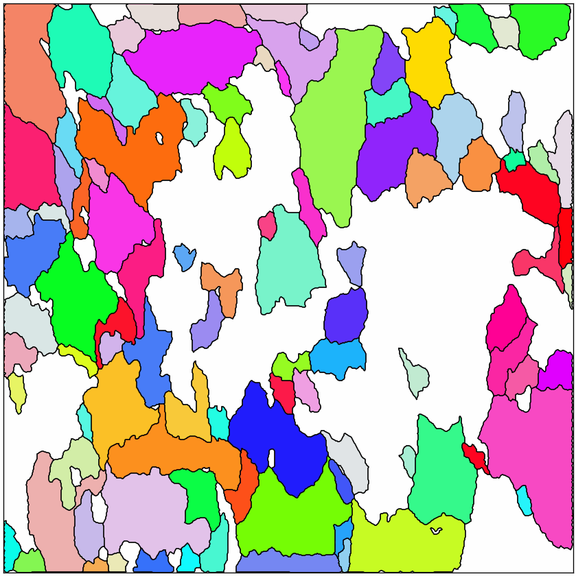
Similar colours do not form one dominant spatial population in this map. The accepted axes also cover much of the fundamental sector rather than gathering at one crystal direction.
Axes in specimen coordinates
A continuous one-to-one colour key cannot cover a whole sphere without a discontinuity. MTEX instead draws specimen axes as compass needles: grey for an axis in the map plane, and split into black and white halves when its ends point out of and into the plane.
plot(grains, GOS / degree, micronbar=False)
mtexColorbar(title='GOS in degree')

hold(True)
plot(grainsLarge[isFibre], GAX_S[isFibre], micronbar=False)
hold(False)
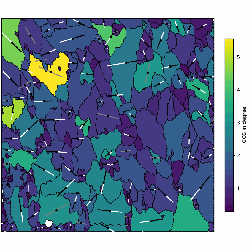
The needles let orientation spread be compared with position and GOS. An axis is not trustworthy merely because a needle can be drawn; only the grains that passed the eigenvalue-ratio screen are shown.
Dispersion axes can relate to flow. Under simple shear they may align with the vorticity axis. Under pure-shear-dominated deformation they may form a girdle whose normal follows the shortening direction. These are kinematic interpretations of an aggregate, not identities that every deformed grain must obey.
plot(GAX_S[isFibre], antipodal=True, markerSize=4)
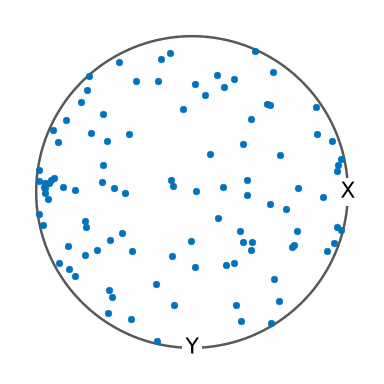
The scatter plot is the direct evidence. Contours make a preferred population easier to judge, but only after axes without a fibre-like orientation cloud have been removed.
Do not weight these contours by fit. A larger fit is a larger distance from the fibre
and therefore a worse fit, not a stronger axis.
axisDensity = calcDensity(GAX_S[isFibre], antipodal=True, halfwidth=10 * degree)
axisDensityMaximum, axisDensityDirection = axisDensity.max()
axisDensityMaximum
4.8582
axisDensityDirection
vector3d (y↓→x)
  antipodal: true
       x        y        z
  -0.994  -0.0439  -0.0999
hold(True)
plot(axisDensity, contour=True, antipodal=True, contours=[1, 2, 3], lineWidth=2)
hold(False)
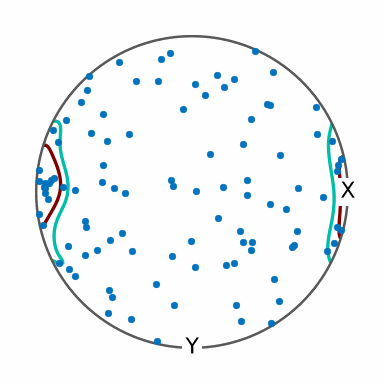
The accepted axes still fill much of the projection, but the distribution is not uniform. Its maximum is 4.86 mrd near the specimen X axis. This supports a preferred population along X rather than one axis shared by every grain, and it does not form a girdle. A flow interpretation also requires the independently established specimen and kinematic frames. This example is ferritic steel rather than a shear-zone rock, so the geological kinematic patterns above are possibilities, not ground truth.
The definitions
Let \(o_{g,i}\) be measurement \(i\) in grain \(g\), and let \(\overline{o}_g\) be the symmetry-aware mean orientation of that grain. MTEX chooses the symmetrically equivalent misorientation with the smallest angle when it computes
\[\mathrm{GROD}_{g,i} = \mathrm{inv}(\overline{o}_g)\,o_{g,i}.\]For \(N_g\) measurements in the grain, the scalar summaries are
\[\mathrm{GOS}_g = \frac{1}{N_g}\sum_i \angle(\mathrm{GROD}_{g,i}),\] \[\mathrm{GAM}_g = \frac{1}{N_g}\sum_i \mathrm{KAM}_{g,i}.\]The neighbour definition inside KAM and the reference orientation inside GROD are therefore part of the definitions, not plotting options.
Further reading
- L. N. Brewer, D. P. Field, and C. C. Merriman, Mapping and Assessing Plastic Deformation Using EBSD, in Electron Backscatter Diffraction in Materials Science, 2nd ed., Springer, 2009, 251-262. This chapter compares the average-misorientation measures and their limitations.
- S. I. Wright, M. M. Nowell, and D. P. Field, A Review of Strain Analysis Using Electron Backscatter Diffraction, Microscopy and Microanalysis 17 (2011), 316-329. It explains why orientation-variation maps should not be read as direct strain maps.
- D. J. Prior, Problems in Determining the Misorientation Axes for Small Angular Misorientations Using Electron Backscatter Diffraction in the SEM, Journal of Microscopy 195 (1999), 217-225. It quantifies the loss of axis precision at small angles.
- W. He, W. Ma, and W. Pantleon, Microstructure of Individual Grains in Cold-Rolled Aluminium from Orientation Inhomogeneities Resolved by Electron Backscattering Diffraction, Materials Science and Engineering A 494 (2008), 21-27. It relates orientation-spread anisotropy and preferred rotation axes within individual grains.
- Z. D. Michels, B. Tikoff, S. C. Kruckenberg, and J. R. Davis, Determining Vorticity Axes from Grain-Scale Dispersion of Crystallographic Orientations, Geology 43 (2015), 803-806. It develops the aggregate crystallographic-vorticity interpretation used in structural geology.
Related pages
Grain Reference Orientation Deviation develops GROD angle and axis maps. Kernel Average Misorientation develops the neighbourhood and threshold choices behind GAM. Dispersion Axes gives the detailed single-grain validation workflow used before interpreting a fitted axis. The next page, Grain Neighbours, changes from properties inside one grain to relationships between adjacent grains.
Technical details
Two small unindexed regions survive the closing here where MATLAB absorbs them, so the
grains are restricted to the indexed ones before the mean orientations are coloured.
fibre.fit(ori, 'local', diagnostics=True) returns MATLAB’s triple; the eigenvalues are
lam[0] to lam[3], so MATLAB’s lambda(2) and lambda(3) read lam[:, 1] and
lam[:, 2] here. calcGrains writes the grain ids into the map and
ebsd.projectIntoFundamentalRegion() returns a new map. The measurements the closing
absorbed keep their notIndexed phase and carry no orientation, so the fit and the
distances skip them. MATLAB’s table is a printed line.
Citing this page.
This page is part of the documentation of
MTEX, a free and open
source MATLAB toolbox for analyzing and modeling crystallographic textures.
It was written by The MTEX Developers and is published at
https://mtex-toolbox.github.io/GrainOrientationParameters_py.html.
If you use MTEX, or reuse text or figures from this page, in your research,
please cite
F. Bachmann, R. Hielscher, H. Schaeben: Texture Analysis with MTEX - Free and Open Source Software Toolbox, Solid State Phenomena 160 (2010), 63-68. 10.4028/www.scientific.net/SSP.160.63
BibTeX
@article{bachmann2010mtex,
  author  = {F. Bachmann and R. Hielscher and H. Schaeben},
  title   = {Texture Analysis with MTEX - Free and Open Source Software Toolbox},
  journal = {Solid State Phenomena},
  volume  = {160},
  pages   = {63-68},
  year    = {2010},
  doi     = {10.4028/www.scientific.net/SSP.160.63},
  url     = {https://doi.org/10.4028/www.scientific.net/SSP.160.63}
}
Other papers describing specific MTEX methods are listed under Publications — please cite the one that best fits your application. The MTEX source code is licensed under the GNU General Public License v2.0; the text and figures of this documentation are licensed under CC BY 4.0, which permits reuse — including by automated systems — provided The MTEX Developers and this page are credited.