Grain Neighbors

Once a map has been divided into grains, it is also a network. Each grain touches a few others, and those connections carry information that a list of grains alone does not. Twins come in touching pairs, recrystallised grains are surrounded by their parent, and a second phase may sit at the corners between three grains of the first.

A grain is a phase-homogeneous, spatially connected region of EBSD measurements produced by segmentation. See Grain Reconstruction for that step and Selecting Grains for the distinction between a grain ID and its position in a list.

The same relationships are represented measurement by measurement by the grain-boundary network. Working with the mean orientations of whole grains is coarser, but much cheaper on a large map. Misorientation Theory introduces the symmetry used when two mean orientations are compared below.

import matplotlib.pyplot as plt
import numpy as np

from mtex import *

# load the sample in its specimen plotting frame
plottingConvention.default('y↑→x')
ebsd = mtexdata('twins')
CS = ebsd.CS

# reconstruct and smooth the grain outlines
grains = calcGrains(ebsd, angle=5 * degree)
grains = smoothBoundary(grains, 5)

# compute the mean-orientation colours without printing a colour-key notice
colorKey = ipfColorKey(grains)
grainColor = colorKey.orientation2color(grains.meanOrientation)

# colour each grain by its mean orientation
plot(grains, grainColor)

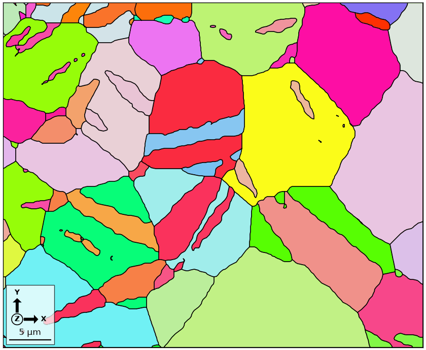
Each coloured region is one reconstructed grain. The narrow regions with colours unlike their surroundings are the twin candidates examined below. Smoothing changes the drawn outlines, but not which grains are neighbours.

Which grain touches which

neighbors returns an \(N \times 2\) array of grain IDs. Each row is one pair of grains that share at least one grain boundary segment. The graph is undirected, so a pair appears only once.

Calling the method on the indexed grains keeps pairs for which both grains are indexed. The outer map rim has a zero on its missing side and therefore does not create a neighbouring-grain pair.

indexedGrains = grains['indexed']
pairs = indexedGrains.neighbors()
pairCount = len(pairs)
pairCount

251

The printed count is the number of unique indexed grain pairs, not the number of boundary segments. A long shared boundary and a short shared boundary each contribute one row.

The values in pairs are persistent IDs rather than positions in indexedGrains. Use an explicit 'id' lookup whenever they select grains. Row 187, for example, identifies the following touching pair.

pairIds = pairs[187]
pairGrains = grains['id', pairIds]

hold(True)
plot(pairGrains.boundary, lineWidth=4, lineColor='b')
hold(False)

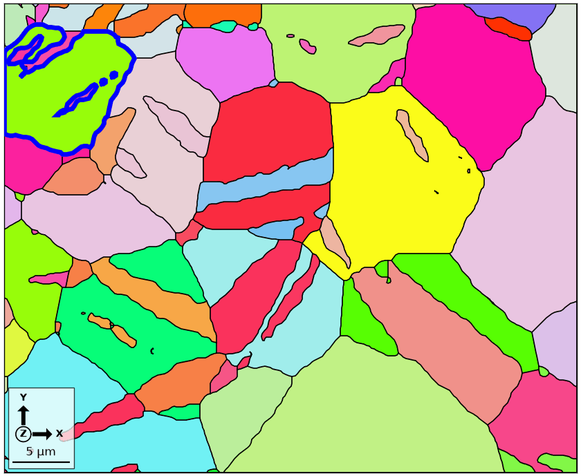
The thick blue outlines enclose the two grains selected by row 187. Their outlines meet along the shared trace that makes them neighbours.

Counting neighbours

numNeighbors counts the distinct grains that touch each grain. It includes neighbours of any phase but does not count the outside of the scanned area as a grain.

The option matrix=True gives the same complete network as a sparse adjacency matrix. Its row and column numbers are persistent grain IDs. For the full grain list it is symmetric because the network is undirected.

adjacency = grains.neighbors(matrix=True)

neighborCount = grains.numNeighbors
plot(grains, neighborCount, micronbar=False)
mtexColorbar(title='number of neighboring grains')

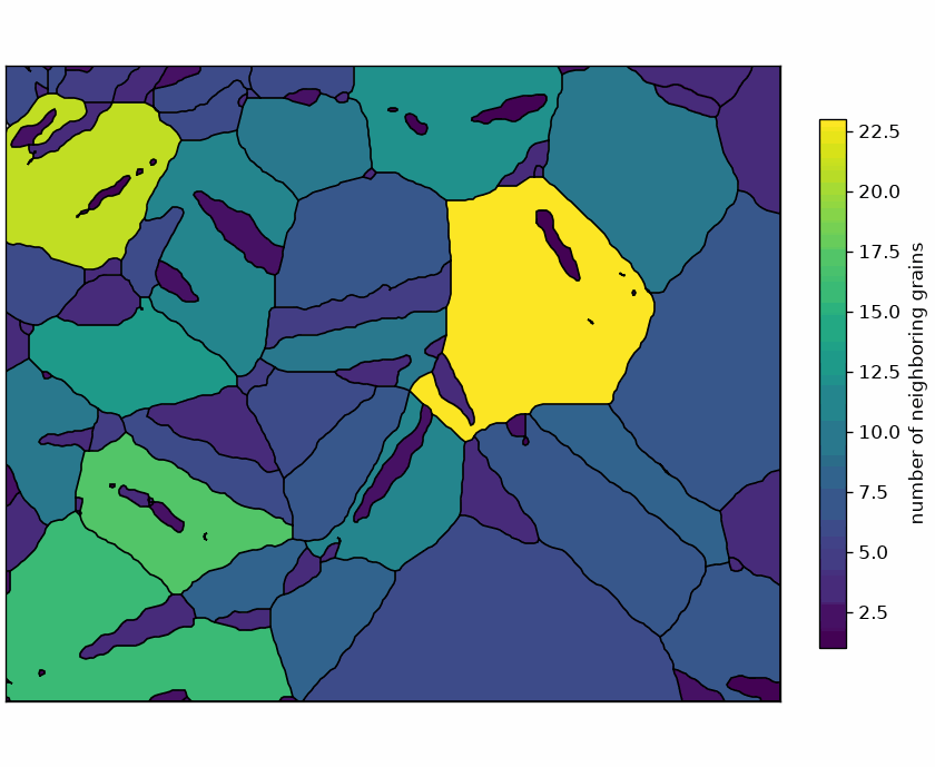
On this map the grains cut by the map edge have the higher counts: they average five neighbours against three and a half for the interior grains. Either count describes only the measured part of the microstructure, just as an observed area or shape does.

One misorientation per neighbouring pair

Two grains that share a boundary have a misorientation. For their mean orientations it is one relationship per pair, rather than one relationship per boundary segment.

A neighbouring pair has no intrinsic first grain. Setting antipodal to true gives its misorientation grain-exchange symmetry, so the relationship and its inverse are equivalent.

mori = pairGrains[0].meanOrientation.inv() * pairGrains[1].meanOrientation
mori.antipodal = True
mori

misorientation (Magnesium → Magnesium)
  antipodal: true
  Bunge Euler angles in degree
  phi1   Phi  phi2
   210  86.8   150

Since the pairs form an array, the same calculation handles every pair at once. Explicit ID lookup keeps the operation correct if the grain list has previously been filtered or reordered.

mori = grains['id', pairs[:, 0]].meanOrientation.inv() * grains['id', pairs[:, 1]].meanOrientation
mori.antipodal = True
mori

misorientation (Magnesium → Magnesium)
  size     : 251
  antipodal: true
  Bunge Euler angles in degree
  phi1   Phi  phi2
  36.4  94.1   355
   330    86   150
   324   168   162
   147  11.8   256
   328  11.1  24.6
     ⋮     ⋮     ⋮
   149  91.3   150
   256  34.1   146
   150  90.3   151
   120   121   236
  28.5  84.1   268

plt.figure()
plt.hist(mori.angle() / degree, bins=np.arange(0, 96, 5))
plt.xlabel('misorientation angle in degrees')

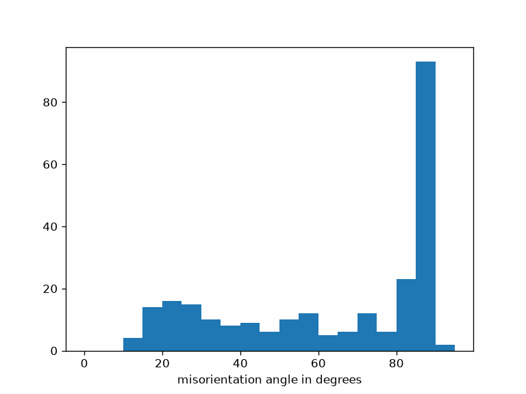
This is a grain-pair-weighted histogram: every neighbouring pair counts once, regardless of its shared trace length or number of segments. A boundary-segment histogram answers a different question.

The result is not the smooth curve expected for a random misorientation distribution. It has a sharp peak in the 85 to 90 degree bin, which in magnesium is the signature of extension twinning.

Finding the twins

A twin relationship is a specific orientation relationship. Here orientation.map constructs it from two pairs of crystallographic vectors that the relationship maps onto each other.

twinning = orientation.map(Miller(0, 1, -1, -2, CS), Miller(0, -1, 1, -2, CS), Miller(2, -1, -1, 0, CS), Miller(2, -1, -1, 0, CS))
twinning

misorientation (Magnesium → Magnesium)
  (01̅12) || (011̅2)   [21̅1̅0] || [21̅1̅0]

twinAngle = twinning.angle() / degree
twinAngle

86.2992

Its disorientation angle is 86.3 degrees, where the peak sits. Angle alone does not identify a twin: unrelated relationships can have the same angle. The comparison below measures distance from the complete crystallographic relationship and uses a 3 degree tolerance.

isTwinning = angle(mori, twinning) < 3 * degree
isPeakBin = (mori.angle() >= 85 * degree) & (mori.angle() < 90 * degree)

numPairs = len(mori)
numTwinPairs = np.count_nonzero(isTwinning)
numPairsInPeak = np.count_nonzero(isPeakBin)
numTwinsInPeak = np.count_nonzero(isTwinning & isPeakBin)
numOtherPairsInPeak = np.count_nonzero(~isTwinning & isPeakBin)

print(f'pairs: {numPairs}, twin pairs: {numTwinPairs} ({100 * numTwinPairs / numPairs:.1f}%), '
      f'pairs in the 85 to 90 bin: {numPairsInPeak}, twins among them: {numTwinsInPeak}, others: {numOtherPairsInPeak}')

pairs: 251, twin pairs: 93 (37.1%), pairs in the 85 to 90 bin: 93, twins among them: 83, others: 10

Of the 251 neighbouring pairs in this map, 93 are within 3 degrees of the twin relationship, or 37 percent. The 85 to 90 degree bin also contains 93 pairs, but the two groups are not identical: 83 are twin matches and 10 are other relationships. The peak is dominated by twins, but angle alone does not select them. Twinning pursues the complete relationship along the boundary segments themselves.

Pairs, and what counts as one

neighbors normally returns a pair only when both grains belong to the list on which it was called. This is why grains['phaseName'].neighbors() returns relationships within one phase and nothing else.

Sometimes the required rule is every pair in which at least one grain belongs to the list. That is how to ask for all neighbours of one grain. The option full=True switches to this rule.

centralId = 92

# get all pairs containing grain ID 92
centralPairs = grains['id', centralId].neighbors(full=True)

# remove the centre ID from the array, leaving its neighbour IDs
neighborIds = centralPairs[centralPairs != centralId]

plot(grains, grainColor, micronbar=False)
hold(True)
plot(grains['id', neighborIds], faceColor='black', alpha=0.5)
plot(grains['id', centralId].boundary, lineColor='white', lineWidth=3)
hold(False)

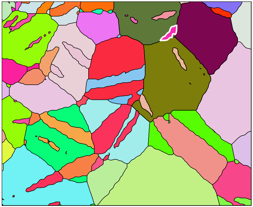
The grain outlined in white has ID 92, and the darkened grains are the grains it touches. Without full=True this list would be empty because no pair has both grains inside a list containing only one grain.

References

• F. Bachmann, R. Hielscher, and H. Schaeben, Grain Detection from 2d and 3d EBSD Data - Specification of the MTEX Algorithm, Ultramicroscopy 111 (2011), 1720-1733. This paper derives the reconstructed grain and boundary network on which the neighbour graph is based.
• J. K. Mason, E. A. Lazar, R. D. MacPherson, and D. J. Srolovitz, Statistical Topology of Cellular Networks in Two and Three Dimensions, Physical Review E 86 (2012), 051128. This paper develops grain-neighbour statistics as a description of cellular microstructures.
• J. W. Christian and S. Mahajan, Deformation Twinning, Progress in Materials Science 39 (1995), 1-157. This review develops deformation-twin crystallography and mechanisms.

Next

Continue with Merging Grains to combine twins with their parent grains. For segment-weighted analysis, continue instead with Misorientations at Grain Boundaries.

Technical details

MATLAB’s table summaries are printed lines here, and the histogram is matplotlib’s plt.hist. Rows of pairs count from zero, so MATLAB’s row 188 is row 187.

@article{bachmann2010mtex,
  author  = {F. Bachmann and R. Hielscher and H. Schaeben},
  title   = {Texture Analysis with MTEX - Free and Open Source Software Toolbox},
  journal = {Solid State Phenomena},
  volume  = {160},
  pages   = {63-68},
  year    = {2010},
  doi     = {10.4028/www.scientific.net/SSP.160.63},
  url     = {https://doi.org/10.4028/www.scientific.net/SSP.160.63}
}