download as script · edit page

An EBSD map records where each measurement was taken and how the crystal there is oriented. Positions and orientations are meaningful together only when they are expressed in the same specimen frame.

A reference frame is the coordinate system in which data are expressed. It has an identity, a basis and a default convention for drawing it. A specimen frame describes the sample, whereas a crystal frame is fixed to a phase’s lattice. Point-group symmetry is attached to a frame but is not the frame itself. See Crystal Reference Frame for that distinction.

An orientation maps a crystal frame into a specimen frame. In an EBSD file its numerical representation is usually a triplet of Euler angles. The positions are \(x\), \(y\) coordinates in the map. If those two parts use different specimen frames, every result that combines them is wrong: a grain shape against its crystal, or a pole figure against the map. The numbers themselves do not reveal the error.

MTEX therefore uses one invariant: the Euler angles refer to the map frame. The \(x\) and \(z\) axes of the map are exactly the axes about which the Bunge Euler rotations are defined. Data that arrives otherwise should be corrected during import.

Read Importing EBSD Data first if EBSD.load is new to you. This page explains the frame decision that import cannot make for you. On Screen Coordinate System Alignment treats plotting conventions in more detail.

from mtex import *

The two specimen frames in a data file

A vendor file may use one specimen frame for map positions and another for Euler angles. The EDAX export dialog shows the mismatch plainly.

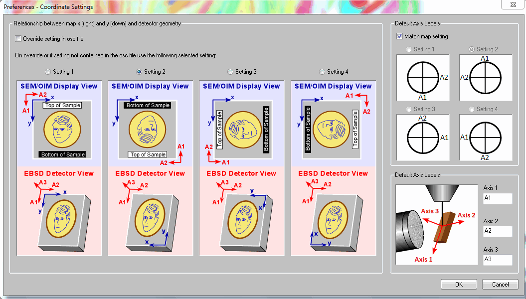
The blue axes \(x\) and \(y\) describe the map coordinates. The red axes \(A_1\), \(A_2\), \(A_3\) describe the frame used by the Euler angles and hence by every pole figure computed from them. None of the four settings makes those axes coincide. Oxford and Bruker files present the same problem with different alignments.

Establish the physical specimen frame before choosing a setting. An asymmetric mark on the sample can link its directions to the SEM image, while a crystal of known orientation checks the link from the diffraction pattern to the lattice. Repeat this calibration when the microscope, detector or acquisition convention changes. Do not choose a correction merely because its map resembles the vendor display.

EDAX numbers the alignments 1 to 4. Setting 2 is by far the most common, but an .ang file does not store the setting. MTEX therefore assumes setting 2 and reports that assumption when none is supplied. State the setting explicitly when it is known, or pass setting=0 when the two frames already coincide and no correction is required.

specimenFrame.specimen.makeDefault()
plottingConvention.default('y↓→x')

ebsd = EBSD.load(mtexdatafile('olivine'), setting=2)

EulerCorrection = ebsd.EulerCorrection
EulerCorrection

rotation
  Bunge Euler angles in degree
  phi1  Phi  phi2
   315  180    45

The displayed rotation is the import’s audit record: it is the correction selected by setting 2. Keeping the object itself silent avoids printing phase and property details that do not answer the frame question.

A format without a numbered catalogue takes the correction directly. EulerCorrection is the rotation that maps the Euler-angle frame onto the map frame:

ebsd = EBSD.load(fileName, eulerCorrection=rotation.map(xvector, xvector, zvector, -zvector))

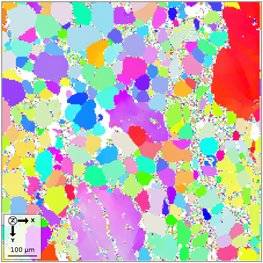
This correction changes the imported orientations so that position and orientation agree. It is not a plotting command. The small indicator in the corner of the following map is switched on by refFrame=True. It states the current screen layout: \(x\) points east, \(y\) south and \(z\) into the screen.

plot(ebsd['olivine'], ebsd['olivine'].orientations, ipfDirection=zvector, refFrame=True)

Screen layout is a different question

A map need not appear on screen as it did in the commercial software. Whether the picture is upside down is a choice of display. Whether the map and orientations are aligned with the specimen is a question of correctness, and only the latter can invalidate the analysis.

A plotting convention states how a reference frame is laid out on screen. It never changes the data. Passing how2plot to one plot changes that plot alone.

# draw x down and y east for this plot only
plot(ebsd['olivine'], ebsd['olivine'].orientations, ipfDirection=zvector, how2plot='x↓→y', refFrame=True)

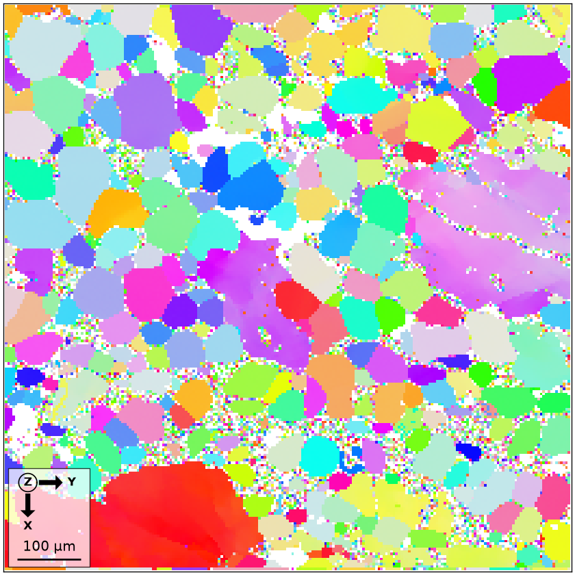
The two screen directions are unchanged, but the axes drawn along them have swapped: \(x\) now runs down and \(y\) to the right. The picture is therefore reflected about the diagonal from top left to bottom right. The large red grain that was at the right edge is now at the bottom left, and the corner indicator has flipped from \(z\) into the screen to \(z\) out of it. Every grain kept its colour, because neither coordinates nor orientations changed.

To change the convention for a whole session, use plottingConvention.default as at the top of this page.

Imported data initially uses the generic specimen frame with axes \(X\), \(Y\), \(Z\). Once their physical meaning is known, the frame can instead be named as a rolling frame with RD, TD, ND, or as a geological frame. See Named Reference Frames for that step.

Check the alignment against the specimen

No value stored in the map can prove that its absolute frame is correct. The check must use independent knowledge of the material or specimen. The most direct test for this olivine map is to draw each large grain’s crystal shape at the measured orientation and compare crystal habit with grain shape.

# reconstruct grains
grains = calcGrains(ebsd)

# use the crystal shape for olivine
cS = crystalShape.olivine()

# select large grains and show the count used below
largeGrains = grains[grains.numPixel > 500]
numLargeGrains = len(largeGrains)
numLargeGrains

# draw the measured orientations and overlay the crystal shapes
plot(ebsd['olivine'], ebsd['olivine'].orientations, refFrame=True, ipfDirection=zvector, location='se')
hold(True)
plot(largeGrains, cS, colored=True)
hold(False)

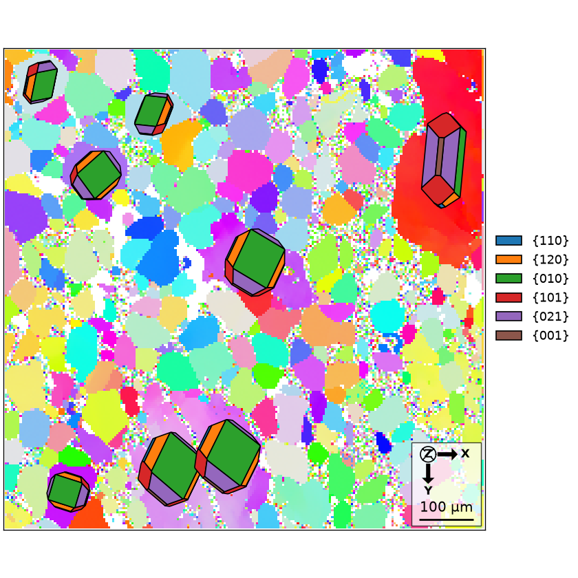
Eight grains pass the size threshold. Most are nearly equant and say little, but the elongated grain at the right edge carries an elongated crystal pointing the same way. That agreement is expected for this rock. It is useful evidence only because the olivine habit is known independently; equant grains or a material without shape-preferred orientation would not provide the same check. A wrong frame would turn or mirror the crystals systematically against the grains.

A second check compares a pole figure with a known specimen direction or feature such as foliation, lineation, RD, TD or ND.

h = Miller([1, 0, 0], [0, 1, 0], [0, 0, 1], ebsd['O'].CS)
plotPF(ebsd['O'].orientations, h, contourf=True)

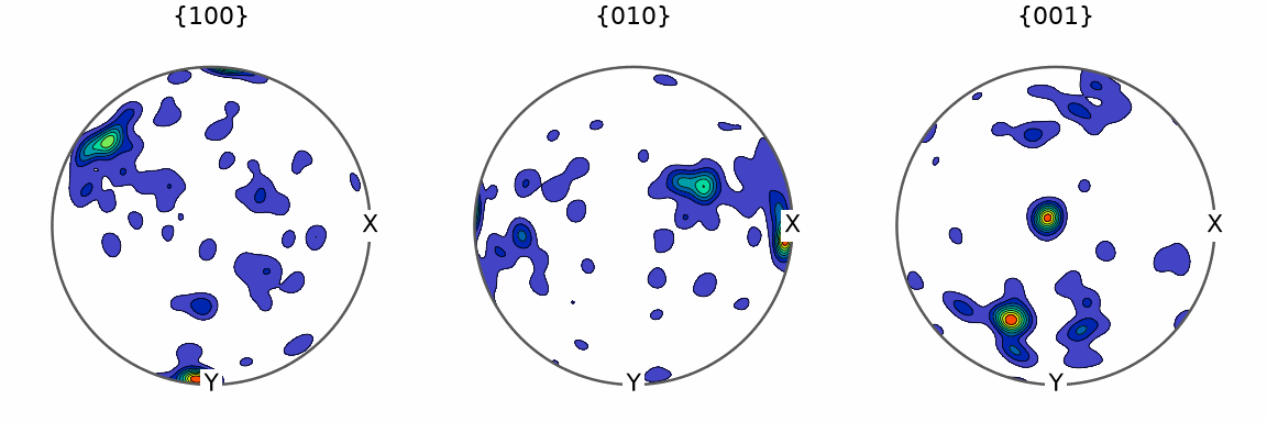
Pole figures describe directions in the specimen, so MTEX draws them in the same frame as the map: \(x\) east and \(y\) south here. A direction read from the map is therefore the same direction in the pole figure. The three plots contain sharp maxima rather than an even covering, so the specimen is textured. The strongest (010) maximum lies on the eastern rim, along the map’s \(x\) axis.

Texture alone does not certify the frame. This maximum becomes a check only when an independent observation says that the corresponding crystal direction should align with that specimen direction.

Change the map coordinates alone

The following three operations are diagnostic demonstrations after a consistent import. They show why an incorrect result can still look ordinary. Rotating only the map coordinates flips or turns the picture while leaving the orientations unchanged. This is useful when the map was recorded mirrored with respect to the specimen.

rot = rotation.byAxisAngle(yvector, 180 * degree)
ebsd_rot = rotate(ebsd, rot, keepEuler=True)

# reconstruct grains
grains = calcGrains(ebsd_rot)

# select only large grains
largeGrains = grains[grains.numPixel > 500]

# put the reference-frame indicator where no crystal covers it
plot(ebsd_rot['olivine'], ebsd_rot['olivine'].orientations, ipfDirection=zvector, refFrame=True, location='ne')

# overlay the crystal shapes
hold(True)
plot(largeGrains, cS, colored=True)
hold(False)

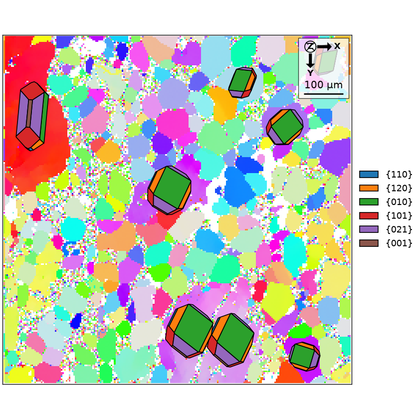
The map is mirrored left to right. The large red grain has moved from the right edge to the left, while each crystal is drawn as before at the mirrored position of its grain. The two frames have been pulled apart on purpose, yet the result still looks like an ordinary map. That is what a wrongly imported data set looks like, and why the correction belongs at import.

Change the Euler angles alone

The opposite operation keeps the coordinates and turns only the orientations.

ebsd_rot = rotate(ebsd, rot, keepXY=True)

# reconstruct grains
grains = calcGrains(ebsd_rot)

# select only large grains
largeGrains = grains[grains.numPixel > 500]

plot(ebsd_rot['olivine'], ebsd_rot['olivine'].orientations, ipfDirection=zvector, refFrame=True, location='se')

# overlay the crystal shapes
hold(True)
plot(largeGrains, cS, colored=True)
hold(False)

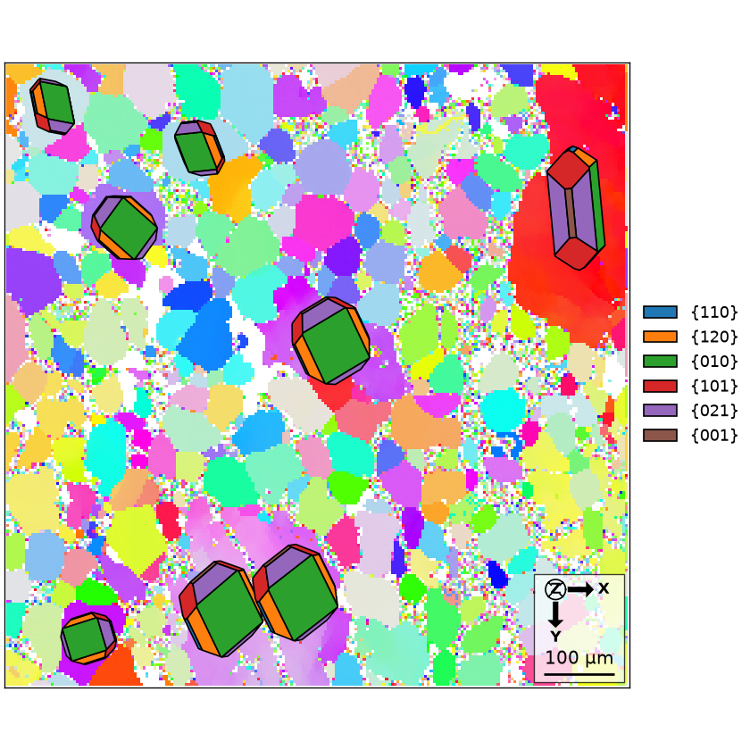
The grains remain where they were, while the crystals turn. The colours do not change: the key asks which crystal direction points along \(z\), this rotation sends that direction to its opposite, and olivine has an inversion centre. Colour alone therefore cannot reveal this frame error. Only a quantity with directional shape can do so.

Rotate coordinates and orientations together

Rotating both parts keeps the data self-consistent and moves the map as a whole. This active rotation is appropriate when the specimen really is to be reoriented by a known amount, for example to correct different mounting angles before several maps are compared. Translation is handled by shift and rotation by rotate.

This is distinct from a frame change, which re-expresses the same physical object in another reference frame without moving it. Naming an already calibrated frame and actively rotating data are not substitutes for one another.

# define a five degree rotation about z
rot = rotation.byAxisAngle(zvector, 5 * degree)

# rotate positions and orientations together
ebsd_rot = rotate(ebsd, rot)

# reconstruct grains
grains = calcGrains(ebsd_rot)

# select only large grains
largeGrains = grains[grains.numPixel > 500]

plot(ebsd_rot['olivine'], ebsd_rot['olivine'].orientations, ipfDirection=zvector, refFrame=True, location='se')

# overlay the crystal shapes
hold(True)
plot(largeGrains, cS, colored=True)
hold(False)

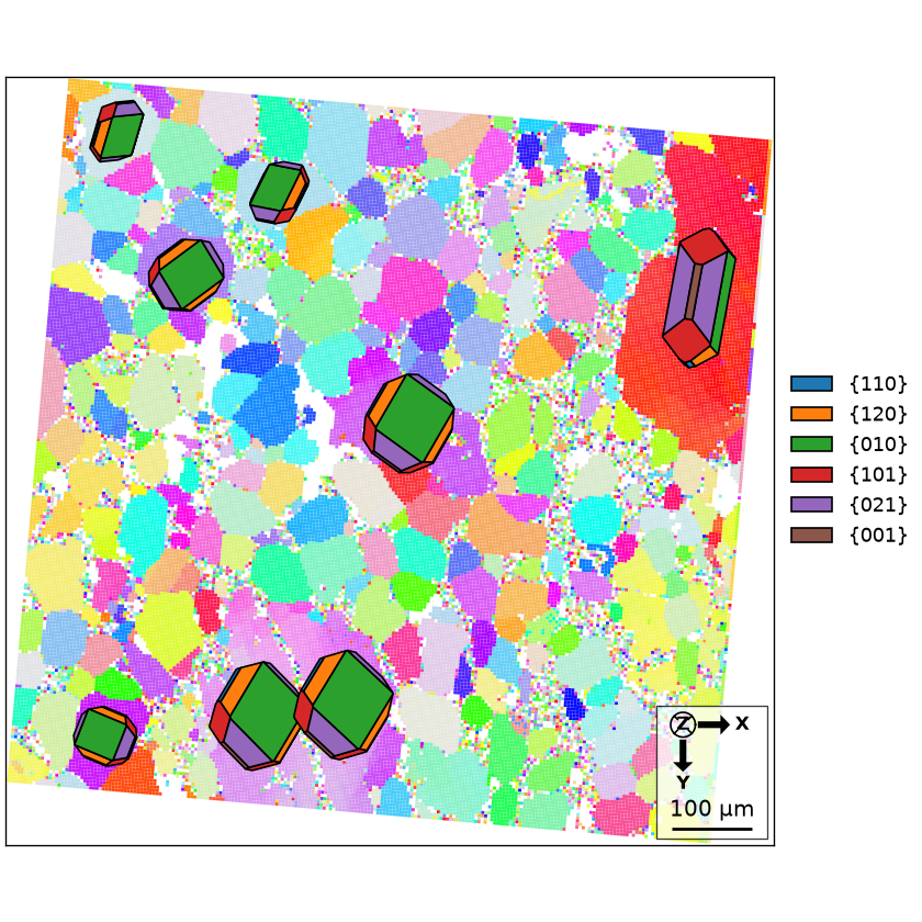
The whole map is tilted by five degrees and the crystals move with it, so they still fit their grains.

The acquisition surface an Oxford file states

Every Oxford format carries one more piece of frame information: the orientation of the surface the map was acquired on, as three Euler angles in degree. A .ctf writes them as AcqE1, AcqE2, AcqE3, a .cpr as the [Acquisition Surface] section, an .h5oina as Specimen Orientation Euler, and Oxford’s own specification defines the quantity as the rotation from the sample surface frame CS1 to the sample primary frame CS0, a frame the user may define on top of it, RD/TD/ND for a rolled sheet, foliation and lineation for a rock. Every .ctf also states, in its header, that its Euler angles refer to CS0; a .cpr keeps them in CS1, the frame the map itself lies in.

Two maps exported both ways, as .cpr/.crc and as .ctf, show what that means in practice.

MEA_ZrB2_60CR_1, AZtec 2023, surface (0, -90, 0): for the same pixel the .crc record holds (315.8, 26.6, 32.8) and the .ctf row (340.25, 23.5, 36.5) degree, while band contrast, slope, bands and MAD agree byte for byte. The two orientations are not symmetrically equivalent; the .ctf one is the .crc one rotated by 90 degree about x, the inverse of the stated surface, to 0.002 degree. The .ctf export had moved the angles into CS0, the .crc had not.
EDXLMDTi64, AZtec 2019, surface (-90, 0, 0): the .crc record and the .ctf row hold identical angles to four decimals, despite the CS0 line in the .ctf header. Nothing was moved.

So the CS0 line of a .ctf is not reliable on its own, and the two files cannot separate the two explanations: the conversion arrived with a newer AZtec, or Oxford moves the angles by the tilt of the surface, its second and third angle, and not by a rotation about the surface normal, the first. The thirteen .h5oina files at hand all state a zero surface, so they add nothing. MTEX follows the second reading, since it fits both pairs: the .ctf loader undoes the tilt of a stated surface and then applies the half turn about y of every Oxford map (X1 west, Y1 south and Z1 out of the surface for a map drawn x east, y south), so that the angles are back in CS1 with the map; a .cpr/.crc is left as it stands; a rotation about the surface normal is never applied. A file with a tilted surface says so in a warning, eulerCorrection overrides the rule, and the surface stays in ebsd.meta['header']. An .h5oina refers its angles to CS0 as well; the loader only reports the value, no file with a non-zero one having been seen.

Reference Frame Alignment