Defining Orientations

An orientation answers one question: how is this crystal placed in this specimen? In MTEX it is a rotation that maps coordinates from the crystal reference frame into the specimen reference frame. It also carries the symmetry attached to each frame.

This page assumes the three-dimensional directions introduced in Defining Three-Dimensional Vectors, the plane and direction notation from Miller Indices, and basic matrix algebra. The constructors are the same as on Defining Rotations, with a crystalFrame supplied as an extra argument.

What this mapping means is developed in Theory and compared with other conventions in MTEX vs. Bunge Convention. This page concentrates on building orientations.

import numpy as np

from mtex import *

plottingConvention.default('y↑→x')

# load the crystal symmetry and reference frame from a CIF file
cs = crystalFrame.load('Cu-Copper.cif')

Euler Angles

Euler angles are the most common input and the one most easily misinterpreted. Their axes, order, and mapping direction belong to the convention. Equal angle triplets in different conventions need not describe the same orientation.

MTEX uses the Bunge convention by default. Naming it explicitly keeps a reusable script independent of the current session preference. Angles are in radians, so values stated in degrees are multiplied by degree.

ori = orientation.byEuler(30 * degree, 50 * degree, 10 * degree, 'Bunge', cs)
ori

orientation (Copper → y↑→x)
  Bunge Euler angles in degree
  phi1  Phi  phi2
    30   50    10

The display gives the three Bunge angles and names the copper crystal symmetry alongside them. This attached crystal frame and symmetry are what distinguish an orientation from a bare rotation.

Rotation Matrix

A \(3 \times 3\) matrix can define the same mapping. Its convention must be checked when it comes from another program: this matrix maps crystal-frame coordinates into specimen-frame coordinates.

M = np.eye(3)

ori = orientation.byMatrix(M, cs)
ori

orientation (Copper → y↑→x)
  Bunge Euler angles in degree
  phi1  Phi  phi2
     0    0     0

The identity matrix gives the orientation in which the Cartesian crystal frame is aligned with the specimen frame. It is the reference setting from which the Euler angles of every other orientation are counted.

The point group does not by itself determine how the Cartesian crystal frame is inscribed into the lattice axes. A statement such as X || a*, Z || c belongs to the crystal reference frame, not to the symmetry. Changing that alignment changes the coordinate description without moving the crystal; see The Crystal Reference System.

Miller Indices

Metallurgy often names an orientation by two crystal quantities: the lattice plane facing the specimen Z axis and the lattice direction pointing along specimen X. The inputs must describe an orthogonal plane normal and direction. That is what orientation.byMiller takes, here for the Goss orientation \((011)[100]\).

ori = orientation.byMiller([0, 1, 1], [1, 0, 0], cs)
ori

orientation (Copper → y↑→x)
  Bunge Euler angles in degree
  phi1  Phi  phi2
     0   45     0

Apply the orientation to the plane normal and the lattice direction to check where they point in the specimen frame.

rPlane = ori * Miller(0, 1, 1, cs, 'hkl')
rDirection = ori * Miller(1, 0, 0, cs, 'uvw')

plot(cat(rPlane, rDirection), upper=True, grid=True, markerSize=10,
     label=['(011)', '[100]'], backgroundColor='w', axisLabels=False)

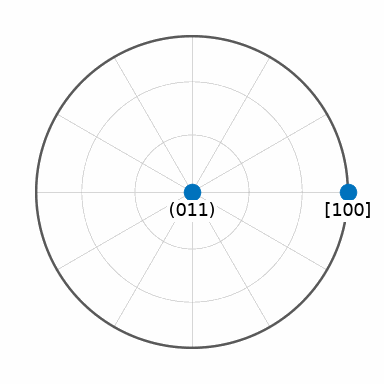
Notice that the \((011)\) pole is at the centre, the specimen Z direction, while \([100]\) is on the specimen X axis at the rim.

Goss and the other named texture components are predefined. The vanishing angular difference confirms that this result is also orientation.goss(cs); see Standard Orientations.

angle(ori, orientation.goss(cs)) / degree

2.6852e-15

Random Orientations

As for rotations, rand generates uniformly distributed orientations and needs the crystal symmetry as well. MTEX stores the 100 results in one vectorized orientation array.

ori = orientation.rand(100, cs)

len(ori)

100

Symmetrically Equivalent Orientations

A crystal cannot distinguish its symmetrically equivalent settings, so an orientation represents a whole class of rotations. symmetrise lists that class.

ori = orientation.byEuler(30 * degree, 50 * degree, 10 * degree, 'Bunge', cs)

len(ori.symmetrise())

24

Copper has point group m-3m with 48 elements, 24 of them proper. Only those 24 describe settings into which the crystal can be physically turned, and they are what symmetrise lists: an orientation is a proper rotation, so the improper half of the point group gives no further orientation.

The improper elements are lattice symmetries all the same, and they act wherever a calculation compares directions rather than orientations - a plane normal and its opposite are the same reflector under Friedel’s law, which is why crystal directions carry antipodal.

The equivalence of the 24 settings is why the angle between two orientations is the smallest angle over all equivalent pairs. The dedicated Symmetry page develops this rule and explains when to use the symmetry=False option.

Specimen Symmetry

A specimen may have symmetry of its own. A rolled sheet, for example, is commonly modelled with orthorhombic symmetry: three mutually perpendicular twofold axes, or equivalently three mirror planes in the full point group. It is represented by a specimenFrame and passed alongside the crystal symmetry.

ss = specimenFrame('orthorhombic')

ori = orientation.byEuler(30 * degree, 50 * degree, 10 * degree, 'Bunge', cs, ss)
ori

orientation (Copper → y↑→x)
  Bunge Euler angles in degree
  phi1  Phi  phi2
    30   50    10

Crystal symmetry acts in the crystal frame and specimen symmetry in the specimen frame, so the class is the product of the two. It holds the 24 proper copper elements times the 4 proper orthorhombic ones.

len(ori.symmetrise())

96

Specimen symmetry is a statement about the sample, not about the measurement. Its axes must match the physical specimen frame, and imposing a symmetry that is not present hides real texture components. Specimen Symmetry explains when to use it.

Technical Details

symmetrise lists the proper equivalents only, ori.CS.numProper() * ori.SS.numProper() of them, where MTEX in MATLAB lists all numSym() * numSym() products of the full point groups and offers a 'proper' option to cut them back. An orientation here is a proper rotation by construction, so the two halves of a Laue group would give each equivalent twice; the improper elements live on the frame and enter through antipodal on the directions instead.

References

• H.-J. Bunge, Texture Analysis in Materials Science: Mathematical Methods, Butterworths, English ed., 1982, establishes the Euler-angle convention used in texture analysis.
• A. Morawiec, Orientations and Rotations: Computations in Crystallographic Textures, Springer, 2004, develops orientations as rotations modulo crystallographic symmetry.
• D. Rowenhorst et al., Consistent representations of and conversions between 3D rotations, Modelling and Simulation in Materials Science and Engineering 23 (2015) 083501, compares conventions and conversion formulas.
• The International Union of Crystallography, Friedel’s law, states the diffraction equivalence and its exception for resonant scattering.

Next

Theory explains how an orientation maps coordinates, which is the definition the rest of MTEX rests on. Pole Figures and Inverse Pole Figures are the two ways of looking at one. Existing orientation files are handled by Import.

@article{bachmann2010mtex,
  author  = {F. Bachmann and R. Hielscher and H. Schaeben},
  title   = {Texture Analysis with MTEX - Free and Open Source Software Toolbox},
  journal = {Solid State Phenomena},
  volume  = {160},
  pages   = {63-68},
  year    = {2010},
  doi     = {10.4028/www.scientific.net/SSP.160.63},
  url     = {https://doi.org/10.4028/www.scientific.net/SSP.160.63}
}