Symmetrically Equivalent Orientations

A crystal cannot distinguish settings related by its point-group symmetry. One physical orientation therefore corresponds to a class of equivalent orthogonal transformations, not to one stored representative. MTEX carries that symmetry with the orientation and uses the whole class in symmetry-aware calculations.

This page assumes that an orientation maps crystal coordinates into specimen coordinates, as developed in Theory. It also assumes the point-group operations introduced in Crystal Symmetries.

A symmetry is the point group under which data are invariant. It is attached to a reference frame, but is not the frame itself. The crystal and specimen symmetries below are therefore attached to opposite sides of the orientation map.

import numpy as np

from mtex import *

plottingConvention.default('y↑→x')

# hexagonal crystal symmetry, with 6 rotations about the c axis
cs = crystalFrame('6')

# specimen symmetry with a twofold axis along z
ss = specimenFrame('112')

# a generic orientation carrying both symmetries
ori = orientation.byEuler(10 * degree, 20 * degree, 30 * degree, 'Bunge', cs, ss)

Which Side Acts

Crystal symmetry acts on the input of the map, from the right. Specimen symmetry acts on its output, from the left. If O represents the stored orientation, every member of its class has the form

The six crystal operations give the following representatives.

# equivalent orientations with respect to crystal symmetry
crystalEquivalents = ori * cs
crystalEquivalents

orientation (6 → y↑→x)
  size: 6
  Bunge Euler angles in degree
  phi1  Phi  phi2
    10   20    30
    10   20    90
    10   20   150
    10   20   210
    10   20   270
    10   20   330

Only the third Euler angle \(\varphi_2\) changes, in steps of \(60^\circ\). In the Bunge convention it is the rotation applied first, in crystal coordinates, which is where the crystal symmetry acts.

Specimen symmetry produces the other kind of equivalence.

# equivalent orientations with respect to specimen symmetry
specimenEquivalents = ss * ori
specimenEquivalents

orientation (6 → y↑→x)
  size: 2
  Bunge Euler angles in degree
  phi1  Phi  phi2
    10   20    30
   190   20    30

Now \(\varphi_1\) changes because it is applied last, in specimen coordinates. Combining both sides gives \(2 \times 6 = 12\) representatives.

allEquivalents = ss * ori * cs
allEquivalents

orientation (6 → y↑→x)
  size: 2 × 6
  Bunge Euler angles in degree
  phi1  Phi  phi2
    10   20    30
    10   20    90
    10   20   150
    10   20   210
    10   20   270
    10   20   330
   190   20    30
   190   20    90
   190   20   150
   190   20   210
   190   20   270
   190   20   330

symmetrise is the shortcut for this product. It returns a new orientation array; it does not alter ori.

classSize = len(symmetrise(ori))
classSize

12

Proper and Improper Operations

Both groups in the first example contain only proper rotations. A full point group may also contain improper operations such as inversion or reflection. An orientation is a proper rotation, so only the proper half of a point group gives another setting of the crystal, and that is the half symmetrise lists. For cubic m-3m symmetry it returns the 24 rigid rotations out of the 48 orthogonal transformations of the group.

cubicOri = orientation.id(crystalFrame('m-3m'))

cubicCount = len(symmetrise(cubicOri))
cubicCount

24

The 24 improper operations remain symmetries of the lattice. They act wherever lattice or diffraction equivalence is the subject, which is a question about directions: a crystal direction reduces over the full group of its frame and carries antipodal for Friedel’s law.

What This Looks Like in a Pole Figure

One orientation and one crystal direction give a family of specimen directions. The complete=True flag keeps both hemispheres visible here so none of the twelve directions is folded into a smaller plotting region.

h = Miller(1, 0, 0, cs)

plotPF(ori, h, complete=True, markerSize=10, figSize='small')

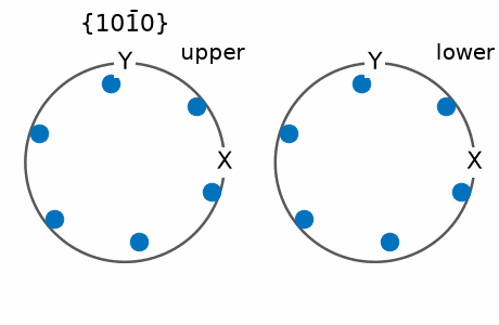
Notice six poles in each hemisphere. The sixfold crystal symmetry creates the crystallographically equivalent direction family, and the twofold specimen symmetry repeats that family in the specimen frame. Without complete=True, plotPF exploits both antipodal equivalence and specimen symmetry and shows only the non-redundant part of this example.

Which member a calculation produces depends on the stored representative. Symmetry-aware comparisons avoid making a physical result depend on that arbitrary choice.

Coincidences

The product of the group sizes is the number of representatives before duplicates are removed. Some orientations make a left-side and a right-side operation describe the same transformation. At the identity orientation the crystal c axis and specimen z axis coincide, so the class has 12 entries but only 6 distinct ones. The unique=True option removes the duplicates.

identityOri = orientation.id(cs, ss)

coincidentCounts = [len(symmetrise(identityOri)), len(symmetrise(identityOri, unique=True))]
coincidentCounts

[12, 6]

Symmetry in Every Comparison

Because the class is what matters, the angle between two orientations is the smallest rotational angle over their equivalent representatives. A fixed probe orientation therefore has the same symmetry-aware angle to every equivalent of the rotation returned by orientation.goss. The named rotation is used only as a reproducible reference here.

probe = orientation.byEuler(37 * degree, 48 * degree, 23 * degree, cs)
referenceEquivalents = symmetrise(orientation.goss(cs))

symmetryAwareAngles = angle(probe, referenceEquivalents) / degree
symmetryAwareAngles

array([28.9235, 28.9235, 28.9235, 28.9235, 28.9235, 28.9235])

Switching symmetry off compares the stored rotations directly. It gives six different angles, whose minimum is the repeated value above.

rawAngles = angle(probe, referenceEquivalents, symmetry=False) / degree
rawAngles

array([ 55.3931,  28.9235,  75.3016, 132.464 , 169.2501, 111.1564])

The symmetry=False flag is implemented by angle, dot, and unique, among other orientation methods. Reach for it when an angle or dot product comes out smaller than expected. Leave it alone otherwise, because the symmetry-aware answer is normally the physically meaningful one.

Do not pass symmetry=False to calcCluster. That method does not define the flag, and an unknown option can be ignored silently.

Technical Details

ori * cs and ss * ori list the equivalents on one side, the group along a new axis, so ss * ori * cs is the full class shaped (2, 6). The elements are the proper ones of each group, as symmetrise uses; an improper element would repeat an equivalent already in the list, an orientation being proper.

References

• A. Morawiec, Orientations and Rotations: Computations in Crystallographic Textures, Springer, 2004, develops orientation space and the effects of crystal and specimen symmetry.
• H.-J. Bunge, Texture Analysis in Materials Science: Mathematical Methods, Butterworths, English ed., 1982, establishes the Euler-angle and orientation conventions used in texture analysis.
• R. Arnold, P. E. Jupp and H. Schaeben, Orientation relationships, orientational variants and the embedding approach, Journal of Applied Crystallography 56 (2023), 725-736, describes crystal orientations as equivalence classes in \(\mathrm{SO}(3)/K\).
• ISO 24173:2024, Microbeam analysis – Guidelines for orientation measurement using electron backscatter diffraction, gives current guidance for reproducible EBSD orientation measurements.

Next

The region of rotation space that holds exactly one member of each class is the Fundamental Region. Symmetry of the specimen, and when it should be imposed at all, is Specimen Symmetry. The same minimum-angle rule becomes central when comparing two crystals in Misorientations.

@article{bachmann2010mtex,
  author  = {F. Bachmann and R. Hielscher and H. Schaeben},
  title   = {Texture Analysis with MTEX - Free and Open Source Software Toolbox},
  journal = {Solid State Phenomena},
  volume  = {160},
  pages   = {63-68},
  year    = {2010},
  doi     = {10.4028/www.scientific.net/SSP.160.63},
  url     = {https://doi.org/10.4028/www.scientific.net/SSP.160.63}
}