Parts of this page are not yet available in Python; the MATLAB page has them all.

download as script · edit page

A notIndexed pixel is a real scan measurement whose diffraction pattern could not be indexed. Patterns measured at grain boundaries may combine signal from both neighbouring grains. Cracks, pores, scratches, surface contamination, or a phase omitted during indexing may also prevent a usable solution.

A missing lattice site is different: no retained measurement occupies that position. This can happen when a scan is interrupted or when selecting or cropping a map leaves an irregular footprint. Both cases appear as missing orientations, but their experimental meanings are not interchangeable.

MTEX can assign orientations to these positions from their neighbours. The assigned values are reconstructions, not measurements. Keep that provenance when the filled map is used for quantitative analysis.

This page assumes familiarity with selecting EBSD data, orientation maps, and grain reconstruction. Reducing random error at positions that already have orientations is the separate subject of Denoising Orientation Maps. Filling also cannot correct an indexed but wrong orientation. The next page, Correcting Pseudo Symmetry, treats one important source of that different error.

import numpy as np

from mtex import *

A complete map for comparison

The first example is an orientation map of ferrite. The object summary reports the indexed ferrite measurements and the sites whose phase is notIndexed: one measurement the indexing rejected, and the 135 sites of the hexagonal lattice the file leaves empty.

# import the data in its measurement frame
plottingConvention.default('y↓→x')
ebsd = mtexdata('ferrite')
ebsd

EBSD (y↓→x)
  size: 270 × 234 grid
  Phase  Orientations  Mineral     Color         Symmetry  Crystal reference frame
  0      1 (0.0016%)   notIndexed
  1      63044 (100%)  Ferrite     LightSkyBlue  m-3m      Ferrite
  properties : ci, fit, iq, sem_signal
  scan unit  : um
  X × Y      : [0 → 69.9] × [0 → 69.89]
  hex lattice: spacing 0.3

# reconstruct the grain structure
grains = calcGrains(ebsd, angle=10 * degree, minPixel=5)

# smooth the pixel staircase of the grain boundaries
grains = smoothBoundary(grains, 5)

# plot the orientation map and its reconstructed grain boundaries
plot(ebsd, ebsd.orientations, ipfDirection=zvector)
hold(True)
plot(grains.boundary, lineWidth=1.5)
hold(False)

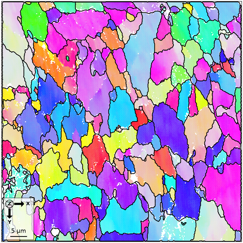
The boundary overlay supplies the geometric constraint used below. It separates missing positions in grain interiors from unresolved corridors along grain boundaries.

A very sparse measured data set

To make the two filling methods easy to compare, we discard approximately 75 percent of the measurements and retain approximately 25 percent. This removes measured positions as well as retaining the notIndexed measurements that happen to be sampled.

ebsdSub = ebsd[np.random.default_rng(0).random(ebsd.size) > 0.75]
ebsdSub

EBSD (y↓→x)
  size: 15770
  Phase  Orientations  Mineral     Color         Symmetry  Crystal reference frame
  0      565 (3.6%)    notIndexed
  1      15179 (96%)   Ferrite     LightSkyBlue  m-3m      Ferrite
  properties : ci, fit, grainId, iq, sem_signal
  scan unit  : um
  X × Y      : [0 → 69.9] × [0 → 69.89]
  hex lattice: spacing 0.3

# plot the retained data
plot(ebsdSub, ebsdSub.orientations, ipfDirection=zvector)

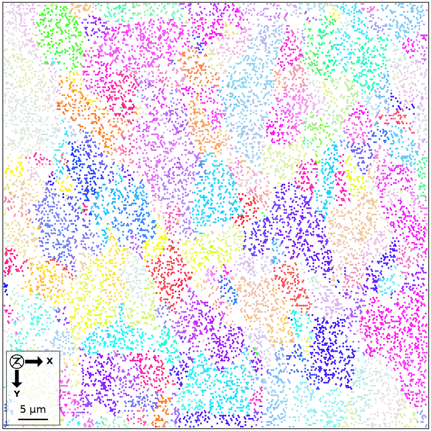
The object summary gives the exact retained counts. The plot now consists of isolated coloured measurements, so the original grain shapes cannot be read from the orientation map alone.

We first reconstruct grains from the retained quarter of the map. The option alpha closes narrow notIndexed regions during segmentation; it does not itself assign orientations. See Grain Reconstruction for that distinction.

# reconstruct the grain structure
grainsSub = calcGrains(ebsdSub, angle=10 * degree, minPixel=5, alpha=15)

grainsSub = smoothBoundary(grainsSub, 5)

hold(True)
plot(grainsSub.boundary, lineWidth=1.5)
hold(False)

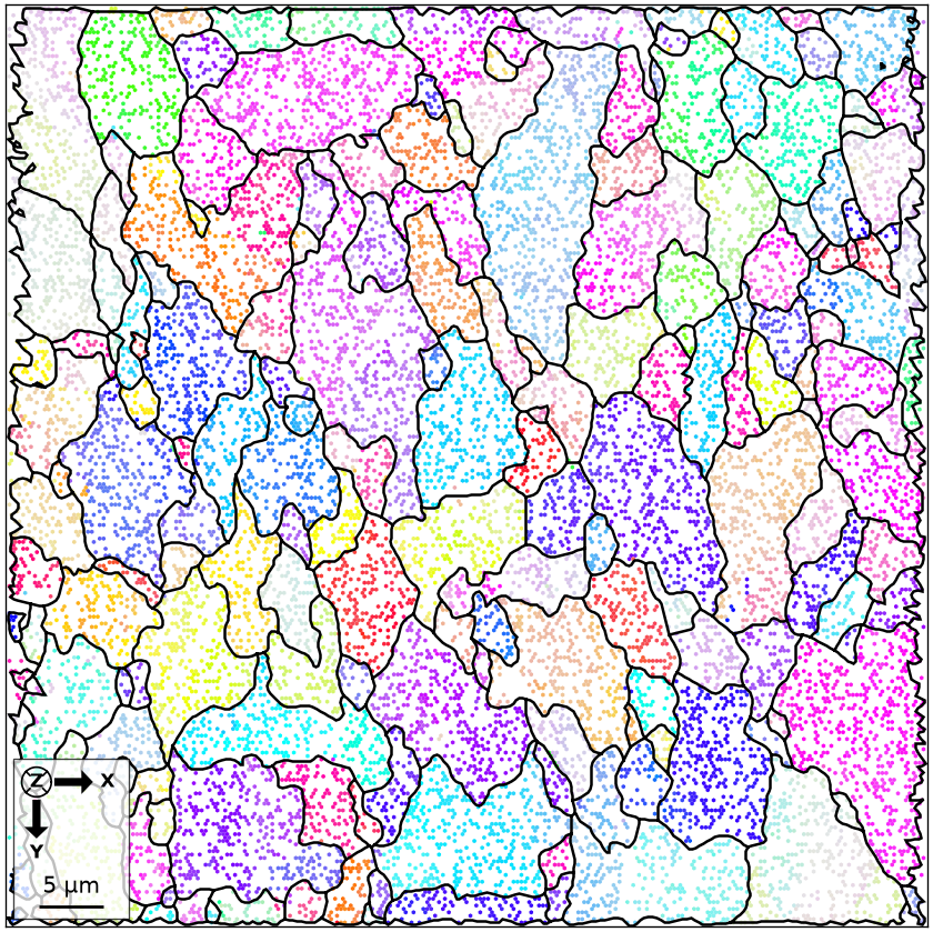
The boundaries recover the main grain outlines despite the sparse input. They also divide the map into interiors that may be filled and boundary corridors that should remain unresolved.

Filling within the grains

fill estimates the missing orientations. Pass the reconstructed grains whenever boundaries are known. MTEX then rejects positions outside every grain and prevents an orientation from being carried across a grain boundary: a position is filled only from the grain whose polygon holds it, and where the measurements of that grain do not reach it, the grain’s mean orientation stands in. gridify first materialises the empty sites of the scan lattice as a matrix-shaped map, which is what fill then fills; it does not change which values are assigned.

ebsdSub_filled = fill(ebsdSub.gridify(), grainsSub)

plot(ebsdSub_filled['indexed'], ebsdSub_filled['indexed'].orientations, ipfDirection=zvector)

hold(True)
plot(grainsSub.boundary, lineWidth=1.5)
hold(False)

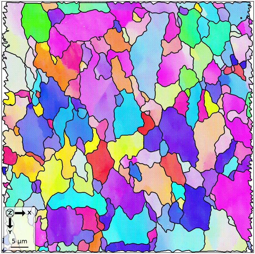
The grain interiors are now coloured. Positions not covered by a grain remain notIndexed, which preserves holes along the grain boundaries. MATLAB’s fill repeats the nearest measurement, which leaves sharp patches; the port continues the orientation field of the grain across the hole, by the edge preserving filter smooth uses.

Filling with a denoising filter

A denoising filter can estimate the missing orientations while smoothing the orientation field. Supply the option fill and the grains to smooth. The halfQuadraticFilter used here is a total-variation method for rotation-valued data; its mathematical basis is described by Bergmann et al. (2016).

In contrast to nearest-neighbour interpolation, the filter can create a smooth transition between the estimated orientations. It is still an estimate, and the reconstructed grain boundaries still constrain it. Neither method reconstructs the grains again. The supplied boundaries remain the segmentation model for the filled map.

F = halfQuadraticFilter()
F.alpha = 0.25

# interpolate and smooth the missing orientations
ebsdSub_smoothed = smooth(ebsdSub.gridify(), F, fill=grainsSub)

plot(ebsdSub_smoothed['indexed'], ebsdSub_smoothed['indexed'].orientations, ipfDirection=zvector)

hold(True)
plot(grainsSub.boundary, lineWidth=1.5)
hold(False)

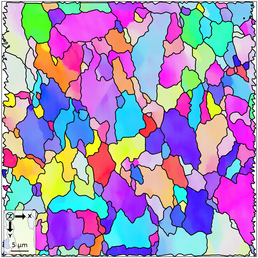
The repeated colour patches have become continuous fields inside the grains. The unfilled corridors still follow the reconstructed boundaries, so the smoother result has not erased the segmentation constraint.

Which data is interpolated

In these grain-constrained calls, both fill and smooth recover the orientation, phase, and grainId of a filled position. The ferrite map carries these properties after filling:

list(ebsdSub_filled.prop)

['iq', 'ci', 'sem_signal', 'fit', 'grainId']

The properties ci, fit, and iq describe the recorded pattern or its indexing solution. The property sem_signal is the simultaneously recorded SEM signal. None has a measured value at a lattice site created by fill. MATLAB leaves each of them as NaN there, so that a reconstructed orientation does not acquire invented evidence of pattern quality; this port solves every floating point property on the same graph as the orientations, so the properties of a filled site are interpolated too.

plot(ebsdSub_filled, ebsdSub_filled.ci)
mtexColorbar(title='confidence index')

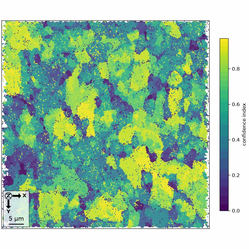
Provenance therefore has to be kept from the ids: a site that was not in the sparse subset has no measured confidence index, whatever the filled map says there. Store such a mask before filling when provenance must be tracked independently.

hasNoMeasuredCI = ~np.isin(ebsdSub_filled.id, ebsdSub.id)
print(f'{np.sum(hasNoMeasuredCI)} of {ebsdSub_filled.size} positions have no measured confidence index')

47410 of 63180 positions have no measured confidence index

MATLAB’s smooth provides a second marker, a per-pixel property named quality set to zero at every position that had no orientation before filtering; it is not ported.

Filling is not resampling

If all per-pixel properties are needed at arbitrary query positions, use interp. It transfers the complete record of the nearest existing measurement to a requested position. The page Interpolating EBSD Data develops that operation.

The requested position must be covered by an existing measurement cell. Thus interp resamples a map but does not fill a hole. Conversely, fill reconstructs missing orientations inside the grains.

A multiphase geological map

Geological samples often contain many notIndexed measurements because of relief, fractures, or phases that are difficult to index. The forsterite example also shows why phase and grain boundaries must constrain filling.

plottingConvention.default('y↑→x')
ebsd = mtexdata('forsterite')
ebsd = ebsd[inpolygon(ebsd, np.array([10, 4, 5, 3]) * 10**3)]

print(f'The submap contains {100 * np.sum(~ebsd.isIndexed) / ebsd.size:.1f} percent notIndexed measurements')

plot(ebsd['Fo'], ebsd['Fo'].orientations, ipfDirection=zvector)
hold(True)
plot(ebsd['En'], ebsd['En'].orientations, ipfDirection=zvector)
plot(ebsd['Di'], ebsd['Di'].orientations, ipfDirection=zvector)

# compute and smooth grains
grains = calcGrains(ebsd, angle=10 * degree, minPixel=3, alpha=3)
grains = smoothBoundary(grains, 5)

# plot the boundary of all grains
plot(grains.boundary, lineWidth=2)
hold(False)

The submap contains 29.0 percent notIndexed measurements

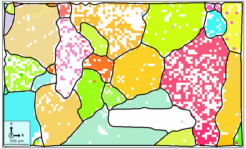
The printed fraction is 29.0 percent, and most of that white is speckle inside the grains. Some grains are peppered with it while their neighbours are almost clean, and 48 percent of all white pixels sit more than one 50 micrometre step from any boundary between two indexed grains. The two large white patches are areas that could not be indexed at all, which segmentation kept as notIndexed grains of their own.

Each phase is drawn with its own IPF key, so a colour identifies an orientation within a phase and not the phase itself. The figure shows where orientations are missing, not which mineral sits where.

The white that does follow the black outlines is the case filling must respect. There the interaction volume straddles two crystals, and giving such a position one neighbour’s orientation would erase the uncertainty that marks the boundary.

Fill only grain interiors

The option fill asks smooth to fill holes inside the grains. Passing grains is what lets MTEX decide whether a position is inside a grain. notIndexed positions along grain boundaries remain untouched.

F = halfQuadraticFilter()
F.alpha = 10

ebsdS = smooth(ebsd, F, fill=grains)

plot(ebsdS['Fo'], ebsdS['Fo'].orientations, ipfDirection=zvector)
hold(True)
plot(ebsdS['En'], ebsdS['En'].orientations, ipfDirection=zvector)
plot(ebsdS['Di'], ebsdS['Di'].orientations, ipfDirection=zvector)

# plot the boundary of all grains
plot(grains.boundary, lineWidth=1.5)
hold(False)

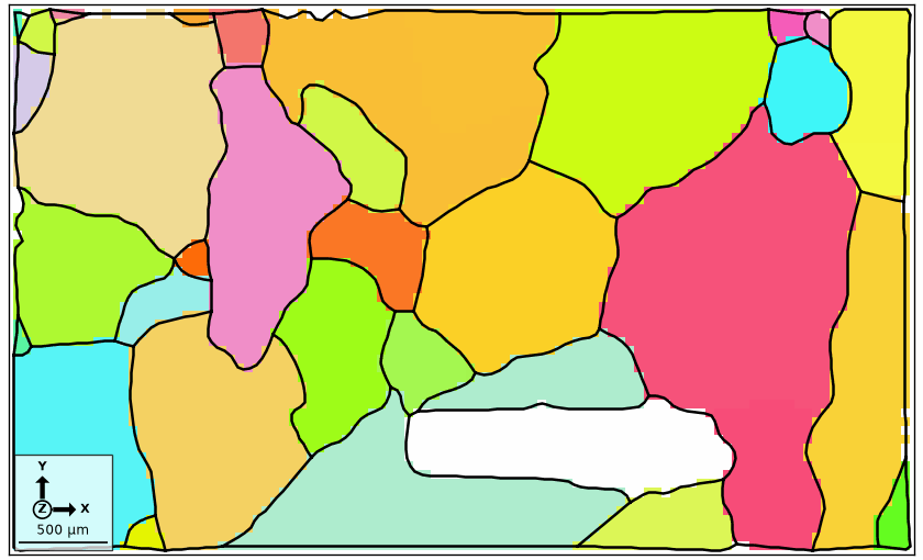
Colour now extends through holes in the grain interiors. The narrow white corridors that remain coincide with reconstructed boundaries, so the filled map does not claim a phase or orientation where the segmentation was deliberately unresolved.

Read the recovered orientation field

Absolute orientation colours can hide small intragranular changes. An axisAngleColorKey compares every orientation with its grain’s mean orientation. The misorientation axis determines the hue, and the angle controls the colour saturation up to the chosen 2.5 degree maximum.

colorKey = axisAngleColorKey(ebsdS['Fo'])
colorKey.oriRef = grains.selectByGrainId(ebsdS['Fo'].grainId).meanOrientation
colorKey.maxAngle = 2.5 * degree

color = colorKey.orientation2color(ebsdS['Fo'].orientations)
plot(ebsdS['Fo'], color, micronbar=False)

hold(True)
colorKey.oriRef = grains.selectByGrainId(ebsdS['En'].grainId).meanOrientation

plot(ebsdS['En'], colorKey.orientation2color(ebsdS['En'].orientations))

# plot boundaries
plot(grains.boundary, lineWidth=4)
plot(grains['En'].boundary, lineWidth=4, lineColor='r')
hold(False)

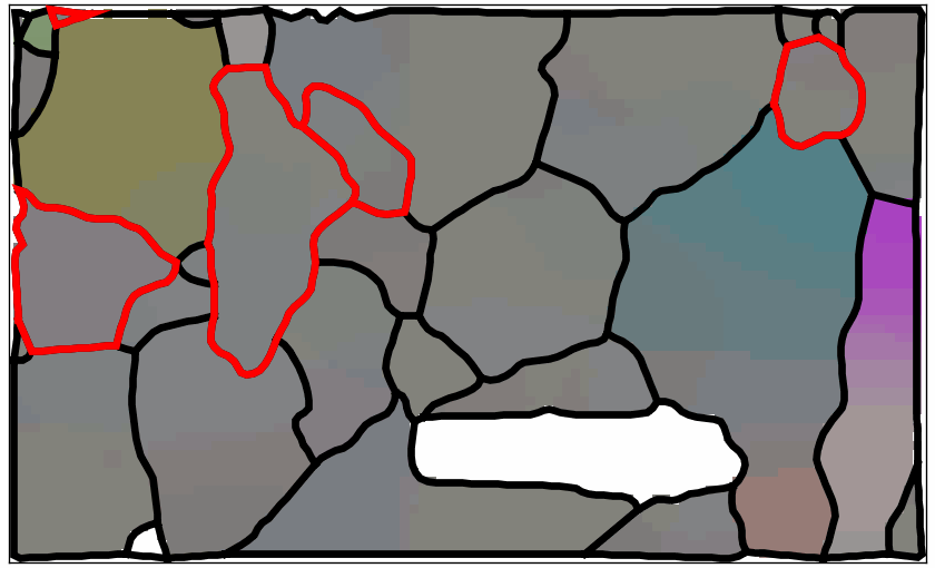
The colour changes smoothly through positions that previously lacked an orientation. This continuity is the filter’s reconstruction of the intragranular orientation gradient, not newly measured deformation.

Compare it with the same view of the original map.

colorKey.oriRef = grains.selectByGrainId(ebsd['Fo'].grainId).meanOrientation
colorKey.maxAngle = 2.5 * degree

color = colorKey.orientation2color(ebsd['Fo'].orientations)
plot(ebsd['Fo'], color, micronbar=False)

hold(True)
colorKey.oriRef = grains.selectByGrainId(ebsd['En'].grainId).meanOrientation

plot(ebsd['En'], colorKey.orientation2color(ebsd['En'].orientations))

# plot boundaries
plot(grains.boundary, lineWidth=4)
plot(grains['En'].boundary, lineWidth=4, lineColor='r')
hold(False)

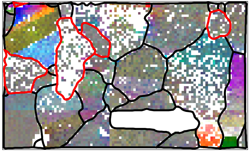
The original view breaks those smooth colour fields with white regions. The comparison shows exactly where filling supplied continuity and guards against reading the reconstructed pixels as independent observations.

Fill Missing Data in Orientation Maps