Select EBSD data

An EBSD variable is a list of measurements. Selecting part of the specimen, one phase, or measurements that satisfy a quality condition is therefore ordinary list indexing. The result is another EBSD variable, so the same phase, position, orientation, and plotting operations apply to it. This is the EBSD version of Lists and Indexing.

Each measurement may also carry a per-pixel property, such as mean angular deviation mad or band contrast bc. A property has one value per measurement and is selected in lockstep with the map; see Properties.

import matplotlib.pyplot as plt
import numpy as np
from matplotlib.patches import Rectangle

from mtex import *

plottingConvention.default('y↑→x')
ebsd = mtexdata('forsterite')

plot(ebsd)

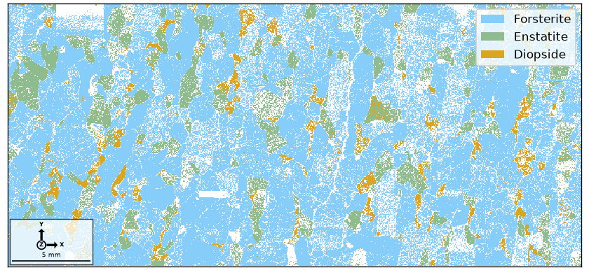
The phase map contains three indexed phases. The white points belong to the notIndexed phase, where a diffraction pattern was recorded but could not be indexed.

Selecting a phase

A mineral name used as an index restricts the list to that phase.

ebsd['Forsterite']

EBSD (y↑→x)
  size: 152345
  Phase  Orientations   Mineral     Color         Symmetry  Crystal reference frame
  1      152345 (100%)  Forsterite  LightSkyBlue  mmm       Forsterite
  properties    : bands, bc, bs, error, mad
  scan unit     : um
  X × Y         : [0 → 3.655e+04] × [0 → 1.675e+04]
  square lattice: spacing 50

Two things in that display are worth noticing. The list is shorter: 152345 of the 245952 measurements are forsterite. Its grid is gone as well. A selection is generally not a full rectangular grid, although every retained measurement still has its original position.

Use gridify when later code explicitly needs a matrix-shaped map. Many spatial MTEX operations reconstruct the virtual lattice internally; Square and Hex Grids explains when the stored grid shape matters.

A prefix of a mineral name works as an abbreviation when it begins one mineral only, so use the full name when two phase names begin alike. Several phases are selected by grouping their names in a list.

ebsd[['Fo', 'En']]

EBSD (y↑→x)
  size: 178403
  Phase  Orientations  Mineral     Color         Symmetry  Crystal reference frame
  1      152345 (85%)  Forsterite  LightSkyBlue  mmm       Forsterite
  2      26058 (15%)   Enstatite   DarkSeaGreen  mmm       Enstatite
  properties    : bands, bc, bs, error, mad
  scan unit     : um
  X × Y         : [0 → 3.655e+04] × [0 → 1.675e+04]
  square lattice: spacing 50

Two names are available whatever the minerals are called. The name 'indexed' selects every point matched to a phase. The degenerate phase 'notIndexed' selects points whose diffraction pattern could not be indexed.

ebsd['indexed']

EBSD (y↑→x)
  size: 187467
  Phase  Orientations  Mineral     Color         Symmetry  Crystal reference frame
  1      152345 (81%)  Forsterite  LightSkyBlue  mmm       Forsterite
  2      26058 (14%)   Enstatite   DarkSeaGreen  mmm       Enstatite
  3      9064 (4.8%)   Diopside    Goldenrod     12/m1     Diopside
  properties    : bands, bc, bs, error, mad
  scan unit     : um
  X × Y         : [0 → 3.655e+04] × [0 → 1.675e+04]
  square lattice: spacing 50

Plotting a phase selection uses the ordinary plot command.

plot(ebsd['Forsterite'], ebsd['Forsterite'].orientations, ipfDirection=zvector)

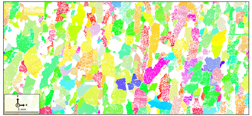
Only the forsterite footprint remains. Its colour still varies with orientation because selection changes the list, not the plotting rule; see Plot.

Restricting to a region of interest

A rectangle is specified as [xmin, ymin, width, height] in the map units, here microns.

region = np.array([5, 2, 10, 5]) * 10**3

Draw the rectangle on the phase map before applying it.

plot(ebsd)
plt.gca().add_patch(Rectangle(region[:2], region[2], region[3], edgecolor='red', linewidth=2, fill=False))

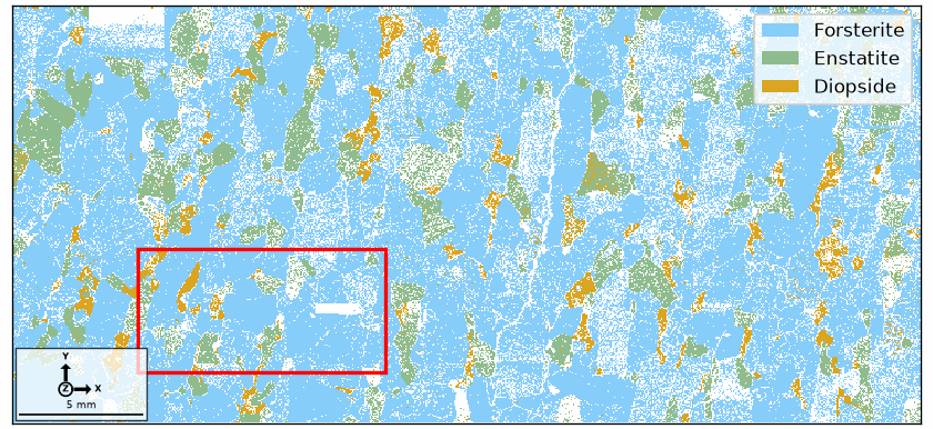
The red rectangle crosses all three indexed phases and many notIndexed points. inpolygon tests every measurement and returns one True or False for each point.

condition = inpolygon(ebsd, region)

Logical indexing keeps the points for which the condition is True: 20301 of the 245952 measurements, about one twelfth of the map.

ebsdRegion = ebsd[condition]
ebsdRegion

EBSD (y↑→x)
  size: 20301
  Phase  Orientations  Mineral     Color         Symmetry  Crystal reference frame
  0      4052 (20%)    notIndexed
  1      14093 (69%)   Forsterite  LightSkyBlue  mmm       Forsterite
  2      1397 (6.9%)   Enstatite   DarkSeaGreen  mmm       Enstatite
  3      759 (3.7%)    Diopside    Goldenrod     12/m1     Diopside
  properties    : bands, bc, bs, error, mad
  scan unit     : um
  X × Y         : [5000 → 1.5e+04] × [2000 → 7000]
  square lattice: spacing 50

Plot the selected region with the same phase colours.

plot(ebsdRegion)

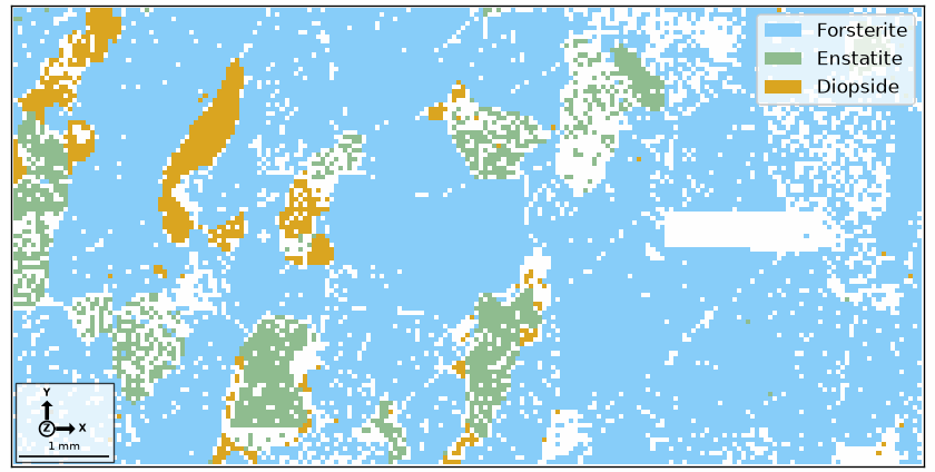
The cropped map keeps its specimen coordinates rather than being moved to the origin. Only its extent and list membership have changed.

A region need not be rectangular. inpolygon also accepts the vertices of any closed polygon.

Screening measurements by fit quality

Indexing software stores quantities that describe the pattern solution. Oxford Channel maps commonly provide the mean angular deviation mad, for which lower values mean a closer angular fit. EDAX OIM maps commonly provide a confidence index ci, for which higher values mean that the winning indexed solution is better separated from the runner-up.

These quantities are not interchangeable measures of orientation error. A threshold flags measurements for scrutiny; it does not prove that an orientation is wrong. Inspect the spatial map and the distribution before choosing a data-dependent threshold.

plot(ebsdRegion, ebsdRegion.mad)
mtexColorbar(title='mean angular deviation (degree)')
setColorRange([0, 1.2])

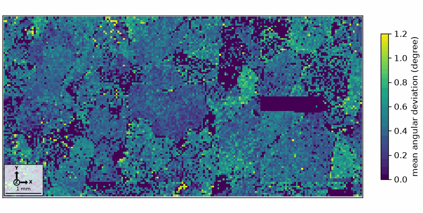
Most of the map sits at about 0.4°. The deep blue patches are the notIndexed points, which report 0. The yellow speckles are the worst fits in this map and lie mainly along grain boundaries, where the interaction volume can contain signal from two crystals. A histogram shows the populations more clearly.

plt.figure()
plt.hist(ebsdRegion.mad, bins=30)
plt.xlabel('mean angular deviation (degree)')

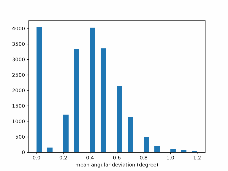
The tallest bar is at zero. It is not a population of perfect fits but the notIndexed points again. The indexed measurements run from 0.1° to 1.2°, with the bulk at 0.4°. A cut at 0.8° removes the tail and keeps 96% of all points in the region.

# take measurements with MAD smaller than 0.8 degrees
ebsdCorrected = ebsdRegion[ebsdRegion.mad < 0.8]
ebsdCorrected

EBSD (y↑→x)
  size: 19420
  Phase  Orientations  Mineral     Color         Symmetry  Crystal reference frame
  0      4052 (21%)    notIndexed
  1      13359 (69%)   Forsterite  LightSkyBlue  mmm       Forsterite
  2      1333 (6.9%)   Enstatite   DarkSeaGreen  mmm       Enstatite
  3      676 (3.5%)    Diopside    Goldenrod     12/m1     Diopside
  properties    : bands, bc, bs, error, mad
  scan unit     : um
  X × Y         : [5000 → 1.5e+04] × [2000 → 7000]
  square lattice: spacing 50

Plot the screened map with the same property on the same colour scale, so that it can be compared with the map above.

plot(ebsdCorrected, ebsdCorrected.mad)
mtexColorbar(title='mean angular deviation (degree)')
setColorRange([0, 1.2])

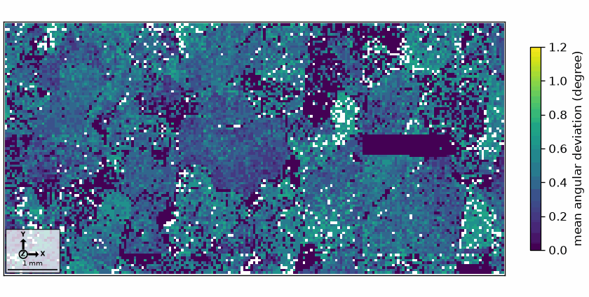
The yellow speckles have gone, because every measurement above 0.8° was removed. Those 881 positions are now empty and render as background.

The deep blue patches are still there, and that is the point to take from this figure. This threshold does not remove notIndexed points: they have no fit to report, so their mad is stored as 0 and passes every smaller-than test. All 4052 notIndexed points are still in the map above.

Dropping them is a separate phase selection. The deliberate output below shows how many indexed measurements remain.

ebsdCorrected['indexed']

EBSD (y↑→x)
  size: 15368
  Phase  Orientations  Mineral     Color         Symmetry  Crystal reference frame
  1      13359 (87%)   Forsterite  LightSkyBlue  mmm       Forsterite
  2      1333 (8.7%)   Enstatite   DarkSeaGreen  mmm       Enstatite
  3      676 (4.4%)    Diopside    Goldenrod     12/m1     Diopside
  properties    : bands, bc, bs, error, mad
  scan unit     : um
  X × Y         : [5000 → 1.5e+04] × [2000 → 7000]
  square lattice: spacing 50

Combining selections

Conditions combine with NumPy’s elementwise & and | operators, or a phase name can narrow a logical selection. This example applies the region and MAD conditions together, then keeps only forsterite.

keep = inpolygon(ebsd, region) & (ebsd.mad < 0.8)
goodForsterite = ebsd[keep]
goodForsterite = goodForsterite['Forsterite']
goodForsterite

EBSD (y↑→x)
  size: 13359
  Phase  Orientations  Mineral     Color         Symmetry  Crystal reference frame
  1      13359 (100%)  Forsterite  LightSkyBlue  mmm       Forsterite
  properties    : bands, bc, bs, error, mad
  scan unit     : um
  X × Y         : [5000 → 1.5e+04] × [2000 → 7000]
  square lattice: spacing 50

Whether notIndexed points should be dropped depends on the analysis that follows. Their locations often record cracks, poor surface preparation, unresolved phases, or difficult grain boundaries. Keep the raw variable and assign a selection to a new name so that this information is not overwritten. Filling Missing Data explains how missing orientations can be treated without pretending they were measured.

Further reading

• A. J. Schwartz, M. Kumar, B. L. Adams and D. P. Field, editors, Electron Backscatter Diffraction in Materials Science, second edition, Springer, 2009, develops the experimental and analytical background to EBSD maps.
• V. Randle, Electron backscatter diffraction: strategies for reliable data acquisition and processing, Materials Characterization 60, 913-922, 2009, reviews acquisition, cleanup, and microstructure analysis choices.
• S. I. Wright et al., Introduction and comparison of new EBSD post-processing methodologies, Ultramicroscopy 159, 81-94, 2015, compares indexing success criteria and shows why their threshold directions depend on the property.
• V. S. Tong et al., The effect of pattern overlap on the accuracy of high resolution electron backscatter diffraction measurements, Ultramicroscopy 155, 62-73, 2015, measures the loss of accuracy caused by overlapping patterns near grain boundaries.
• ISO 24173:2024, Microbeam analysis - Guidelines for orientation measurement using electron backscatter diffraction, gives current guidance for reliable and reproducible EBSD orientation measurements.

Next

Select by Index distinguishes list position, persistent measurement id, map coordinates, and grid indices. Square and Hex Grids explains when to restore matrix shape. Continue with Grain Reconstruction before selecting whole grains rather than individual measurements.

@article{bachmann2010mtex,
  author  = {F. Bachmann and R. Hielscher and H. Schaeben},
  title   = {Texture Analysis with MTEX - Free and Open Source Software Toolbox},
  journal = {Solid State Phenomena},
  volume  = {160},
  pages   = {63-68},
  year    = {2010},
  doi     = {10.4028/www.scientific.net/SSP.160.63},
  url     = {https://doi.org/10.4028/www.scientific.net/SSP.160.63}
}