download as script · edit page

A single EBSD measurement has several addresses. It has a position in a list, an id inherited from its parent map, and a position on the specimen. On a gridded map it also has a row and column. A hexagonal grid offers cube coordinates as a fifth address. They simplify neighbour-based algorithms.

These addresses answer different questions and stop agreeing as soon as measurements are selected or rearranged. This page keeps them apart. See Selecting EBSD Data for phase, property, and region selections. Square and Hex Grids gives the complete gridding model.

import matplotlib.pyplot as plt
import numpy as np

from mtex import *

plottingConvention.default('y↑→x')
ebsd = mtexdata('twins')
ebsd

EBSD (y↑→x)
  size: 137 × 167 grid
  Phase  Orientations  Mineral     Color         Symmetry  Crystal reference frame
  0      46 (0.2%)     notIndexed
  1      22833 (100%)  Magnesium   LightSkyBlue  6/mmm     Magnesium
  properties    : bands, bc, bs, error, mad
  scan unit     : um
  X × Y         : [0 → 49.8] × [0 → 40.8]
  square lattice: spacing 0.3

List position

The summary above identifies the imported map as a square grid. It is already stored as a matrix. Restricting it to a small rectangle returns a plain list. An arbitrary selection is not generally rectangular.

poly = [44, 0, 4, 2]
ebsd = ebsd[inpolygon(ebsd, poly)]
ebsd

EBSD (y↑→x)
  size: 98
  Phase  Orientations  Mineral    Color         Symmetry  Crystal reference frame
  1      98 (100%)     Magnesium  LightSkyBlue  6/mmm     Magnesium
  properties    : bands, bc, bs, error, mad
  scan unit     : um
  X × Y         : [44.1 → 48] × [0 → 1.8]
  square lattice: spacing 0.3

The summary reports 98 measurements. Each coloured square below is one entry in that list. Writing the list position into every square reveals the order in which the entries are stored.

plot(ebsd, ebsd.orientations, ipfDirection=zvector, micronbar=False, edgeColor='k', backend='patch')
text(ebsd, np.arange(len(ebsd)))

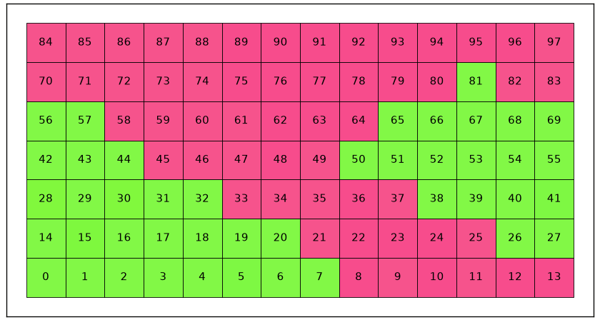
A single numeric subscript selects by list position, counted from zero. The red outline marks entries 15 to 17.

hold(True)
plot(ebsd[15:18], edgeColor='red', faceColor='none', lineWidth=4, backend='patch', legend=False)
hold(False)

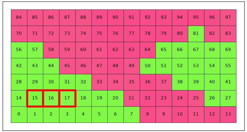
This crop came from a gridded map and inherited its linear order. NumPy advances through every column of one matrix row before moving to the next row. Here that means visiting all x positions at one y position before moving to the next y position. A list imported without gridding instead follows the order in which its measurements were loaded.

Measurement id

Cropping changed every measurement’s position in the list. Entry 15 of the crop was not entry 15 of the full map. Its identifier in that parent map is stored in ebsd.id.

plot(ebsd, ebsd.orientations, ipfDirection=zvector, micronbar=False, edgeColor='k', backend='patch')
text(ebsd, ebsd.id)

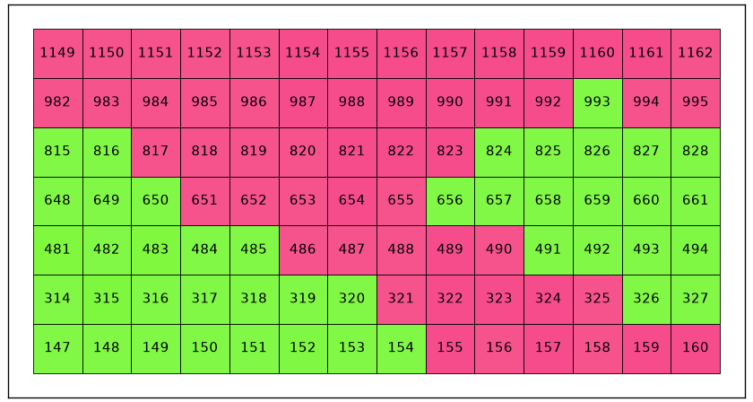
The key 'id' selects by those identifiers. It therefore highlights the same three measurements as the list-position selection above.

hold(True)
plot(ebsd['id', ebsd.id[15:18]], edgeColor='red', faceColor='none', lineWidth=4, backend='patch', legend=False)
hold(False)

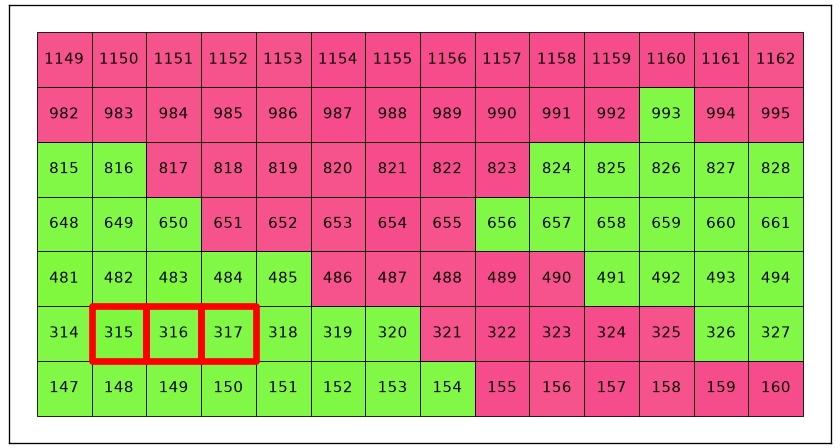
Keep an id when a result from one selection must be matched to another selection from the same parent map. Selection preserves it. Gridding is a different operation. It may assign identifiers for the new raster and stores the input identifiers in oldId. An id is therefore not necessarily a line number in the imported file. See Square and Hex Grids.

Position on the specimen

The key 'xy' returns the measurement closest to a specimen position. Its output shows both the selected id and the actual coordinates.

ebsd['xy', 44.5, 1]

EBSD (y↑→x)
  size: 1
  Phase  Orientations  Mineral    Color         Symmetry  Crystal reference frame
  1      1 (100%)      Magnesium  LightSkyBlue  6/mmm     Magnesium
   Id  Phase             orientation  bands   bc   bs  error  mad
  649      1  (176.5°,104.1°,182.9°)     10  139  245      0  0.5
  scan unit     : um
  X × Y         : [44.4 → 44.4] × [0.9 → 0.9]
  square lattice: spacing 0.3

The expression ebsd[x, y] does not perform that lookup on a plain list; it is an error. On a gridded map the same expression means the pixel in row x and column y. Requiring 'xy' prevents one line from changing meaning when a map changes between list and matrix storage.

Square-grid subscripts

Although the crop is a list, its measurements lie on a regular grid. gridify restores the matrix shape. The shape confirms that this crop has 7 rows and 14 columns.

ebsd = ebsd.gridify()
ebsd.shape

(7, 14)

The labels now show (row, column) rather than a single linear index.

plot(ebsd, ebsd.orientations, ipfDirection=zvector, micronbar=False, edgeColor='black', backend='patch')

i, j = np.indices(ebsd.shape)
labels = [f'({a},{b})' for a, b in zip(i.ravel(), j.ravel())]
text(ebsd, labels)

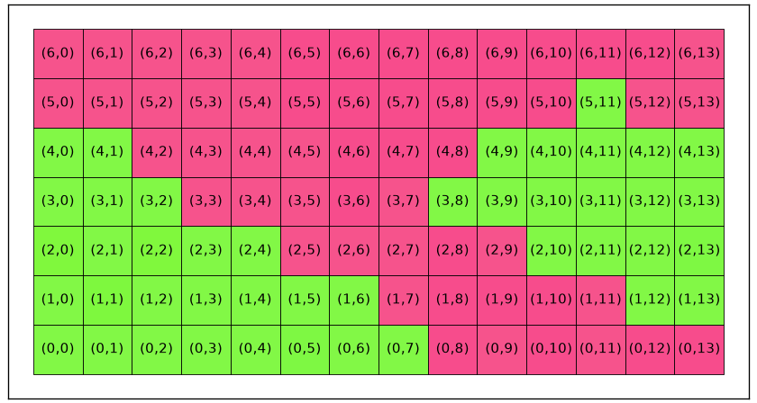
Two subscripts select by row and column. Ranges select a whole row or a rectangular block; the red outline marks columns 1 to 3 of row 1.

hold(True)
plot(ebsd[1, 1:4], edgeColor='red', faceColor='none', lineWidth=4, backend='patch', legend=False)
hold(False)

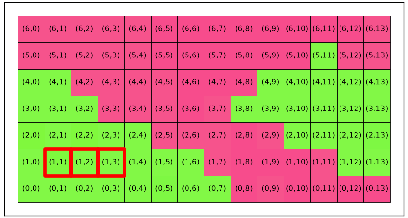
gridify is allowed to reorder a plain list so that dimension 0 follows increasing specimen y and dimension 1 increasing x. This crop is a special case: it already inherited that order from the full gridded map, so its sequence does not change. For a general list, use oldId, which relates input order to raster order. Square and Hex Grids works through that translation.

Hexagonal grids

The same distinction between linear index, id, specimen position, and matrix subscripts applies to a hexagonal measurement grid. The summary below identifies this map as a hexagonal grid. It is stored as a matrix from the start.

plottingConvention.default('y↓→x')
ebsd = mtexdata('titanium')
ebsd

EBSD (y↓→x)
  size: 97 × 84 grid
  Phase  Orientations  Mineral           Color         Symmetry  Crystal reference frame
  1      8100 (100%)   Titanium (Alpha)  LightSkyBlue  622       Titanium (Alpha)
  properties : ci, grainid, iq, sem_signal
  scan unit  : um
  X × Y      : [0 → 996] × [0 → 997.7]
  hex lattice: spacing 12

Row and column indexing works as in the square case. We retain a small block so that its subscripts remain legible.

ebsd = ebsd[9:16, 67:79]

plot(ebsd, ebsd.orientations, ipfDirection=zvector, edgeColor='k', micronbar=False, backend='patch')
plt.axis('off')

i, j = np.indices(ebsd.shape)
labels = [f'({a},{b})' for a, b in zip(i.ravel(), j.ravel())]
text(ebsd, labels)

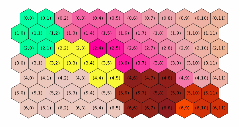
The labels show that rows are horizontal lines of cells. Because alternate rows are offset, a matrix column follows a zigzag rather than a straight line on the specimen.

Cube coordinates

Offset rows make a neighbour step depend on whether the row is even or odd. Cube coordinates replace row and column by three redundant indices, making the six neighbour steps identical everywhere on the grid. They are cell addresses for algorithms, not specimen coordinates.

hex2cube and cube2hex convert between the two systems. Hexagonal Grids explains the geometric construction and further algorithms.

plot(ebsd, ebsd.orientations, ipfDirection=zvector, edgeColor='k', micronbar=False, backend='patch')
plt.axis('off')

x, y, z = ebsd.hex2cube(i, j)
labels = [f'({a},{b},{c})' for a, b, c in zip(*(np.rint(v).astype(int).ravel() for v in (x, y, z)))]
text(ebsd, labels, fontSize=6)

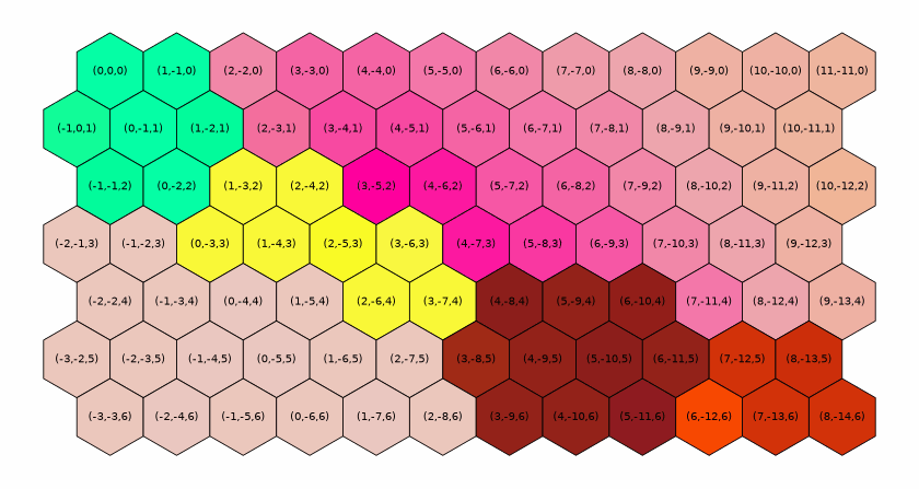
Every displayed triple satisfies \(x + y + z = 0\). A step to any of the six neighbours adds one to one coordinate and subtracts one from another, leaving the third unchanged.

Indexing EBSD Data