Lists and Indexing

Almost every MTEX variable is a list of objects of one kind. An EBSD variable is a list of measurements, a grain2d variable is a list of grains, and grains.boundary is a list of grain boundary segments. An orientation variable commonly stores a list of orientations.

There is no separate type for one grain. A single grain is a grain2d list with length one.

Two consequences account for most list operations in MTEX.

• An elementwise function or property acts on every list element. It usually returns one result per element: grains.area gives one area per grain, and ori.angle() gives one angle per orientation. Reduction functions such as mean are exceptions because they combine several elements into one result. Loops are therefore almost never needed for elementwise calculations.
• Square bracket indexing selects elements as it does for a NumPy array. The result is a list of the same kind, so an operation that accepts the complete list also accepts the selection.

The diagram compares the two main forms of indexing. Position indices pick specified list entries in the requested order. A logical condition keeps the entries whose mask value is true.

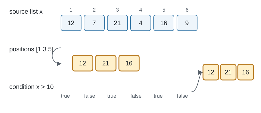
The sections that follow show the indexing itself on plain numbers, for clarity. The same two forms then apply unchanged to any MTEX list.

import numpy as np

Make a list

np.array creates a list by placing values next to one another.

x = np.array([1, 2, 3, 4, 5, 6])
x

array([1, 2, 3, 4, 5, 6])

np.arange is shorthand for a regularly spaced range. With no step specified, it uses a step of one. Its end is exclusive, so the range 1 to 10 is np.arange(1, 11).

x = np.arange(1, 11)
x

array([ 1,  2,  3,  4,  5,  6,  7,  8,  9, 10])

Apply an operation to every element

NumPy applies arithmetic operations elementwise. x**2 squares every element of x independently; a matrix power is np.linalg.matrix_power.

y = x**2
y

array([  1,   4,   9,  16,  25,  36,  49,  64,  81, 100])

Select by position

A list of positions selects those elements in the given order. Here, ind selects the first, third, and fifth squared values. Python counts positions from zero, so the first element has position 0.

ind = [0, 2, 4]
ind

[0, 2, 4]

y[ind]

array([ 1,  9, 25])

Select by condition

A condition evaluated for the complete list returns one logical value per element. A logical value is either true or false. It can be used as an index to retain only the corresponding true entries.

cond = x % 2 == 0
cond

array([False,  True, False,  True, False,  True, False,  True, False,
        True])

y[cond]

array([  4,  16,  36,  64, 100])

The condition tests which values in x are even. Using the same mask to index y returns their squares. This works because x and y have the same length and order.

Use the same pattern with MTEX objects

Nearly every MTEX selection has the same form. For example, grains[grains.area > 100] selects grains with area greater than 100, ebsd[ebsd.mad < 1] selects measurements with a mean angular deviation below 1, and gB[gB.misorientation.angle() > 10*degree] selects grain boundary segments with a misorientation angle greater than 10 degrees.

In each expression, MTEX computes one property value per object. The comparison turns those values into a logical mask, and the brackets apply the mask to the original list.

MTEX also provides two domain-specific selectors. A phase name selects all measurements of that phase, as in ebsd['Forsterite']. For spatial data, a position selects the object found there, as in grains(x, y). See Selecting Grains for spatial grain selections.

References

• NumPy, Indexing on ndarrays, NumPy documentation. It defines positional and boolean indexing and describes the array rules used on this page. The MATLAB page cites MathWorks’ Array Indexing.

Next

Continue with Configuration to learn how session preferences control display, computation, and plotting defaults.

Technical Details

MATLAB counts from one and its ranges 1:10 include the end; Python counts from zero and np.arange(1, 11) excludes it. The values and the selections are MATLAB’s, the positions one less. A map read from a regular grid is a two-dimensional list in the port, so ebsd[ebsd.mad < 1] returns the selected measurements as a one-dimensional list, as NumPy does for a boolean mask.

@article{bachmann2010mtex,
  author  = {F. Bachmann and R. Hielscher and H. Schaeben},
  title   = {Texture Analysis with MTEX - Free and Open Source Software Toolbox},
  journal = {Solid State Phenomena},
  volume  = {160},
  pages   = {63-68},
  year    = {2010},
  doi     = {10.4028/www.scientific.net/SSP.160.63},
  url     = {https://doi.org/10.4028/www.scientific.net/SSP.160.63}
}