Properties

A property stores one value for every element of an MTEX list. When you select, sort, or concatenate the list, MTEX carries those values along in lockstep. This link between an object and its per-element data makes a property useful for filtering, colouring, and later calculations.

List-like classes include EBSD, grain2d, grainBoundary, and PoleFigure. For an EBSD map, a property has one value per measurement point. The expression ebsd[condition].mad therefore returns exactly the MAD values at the selected points.

Properties are not options

A command option changes one command call. It is not stored as per-element data. By contrast, EBSD properties live in ebsd.prop and are resized whenever ebsd[ind] selects part of the map.

Scan-level values live in ebsd.meta, MATLAB’s ebsd.opt. They do not have one value per measurement point and are not resized when the map is subset. This distinction is the test to use: per-point data belongs in prop, while whole-scan data belongs in meta.

Inspecting imported properties

The available properties depend on the data source. An EBSD file usually contributes a confidence measure and an error-of-fit measure. Importers also preserve unrecognised per-point columns as properties.

Load the forsterite example and display the fields collected in prop.

from mtex import *

plottingConvention.default('y↑→x')
ebsd = mtexdata('forsterite', verbose=False)

ebsd.prop

bands: [336×732 float64]
error: [336×732 float64]
  mad: [336×732 float64]
   bc: [336×732 float64]
   bs: [336×732 float64]

Each property may also be read as though it were a regular field of the object. Here the first five MAD values are read as ebsd.mad. The map was read from a regular grid, so its properties are two-dimensional arrays; ravel() lists them in the order of the file.

ebsd.mad.ravel()[:5]

array([0.1, 0.1, 0.1, 0.3, 0.2])

Subsetting keeps values aligned

Select every measurement whose MAD is below one. The two lengths printed below are equal because selecting EBSD points also selects the matching property values.

ebsdSub = ebsd[ebsd.mad < 1]

len(ebsdSub)

242352

len(ebsdSub.mad)

242352

Adding a property

Create a property by assigning to a new field of the map. Any name that is not already a field of EBSD becomes a property, and the assignment checks that the value has one entry per measurement. MATLAB requires the prop part for the first assignment, ebsd.prop.myQuality = ..., because it cannot distinguish a new name from a typo; the port tells them apart by the length of the value.

This example turns MAD into a quality score that decreases as MAD grows.

ebsd.myQuality = 1 / (1 + ebsd.mad)

ebsd.prop

    bands: [336×732 float64]
    error: [336×732 float64]
      mad: [336×732 float64]
       bc: [336×732 float64]
       bs: [336×732 float64]
myQuality: [336×732 float64]

Once the field exists, it can be read or overwritten as ebsd.myQuality. It also survives indexing. The following values belong only to the selected forsterite points.

ebsd['Forsterite'].myQuality[:5]

array([0.9091, 0.9091, 0.9091, 0.7692, 0.8333])

Plotting a property

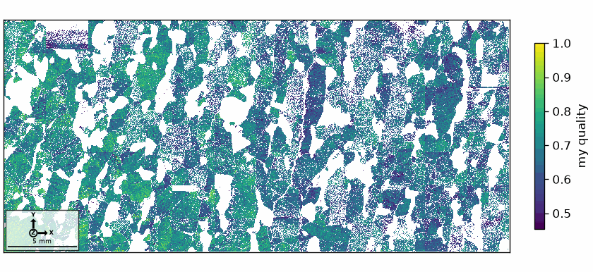
A numeric property can supply one colour value per point. The map shows lower myQuality where MAD is larger and higher myQuality where MAD is smaller; the colours remain attached to the correct measurement points.

newMtexFigure()
plot(ebsd['Forsterite'], ebsd['Forsterite'].myQuality)
mtexColorbar(title='my quality')

Properties may store MTEX objects

A property does not have to be numeric. Any value that supports indexing can be stored. The next property contains one vector3d per forsterite point. Each vector is the specimen direction of that point’s crystallographic \(c\) axis.

ebsdFo = ebsd['Forsterite']
ebsdFo.myAxis = ebsdFo.orientations * Miller(0, 0, 1, ebsdFo.CS)

ebsdFo.prop

    bands: [152345 float64]
    error: [152345 float64]
      mad: [152345 float64]
       bc: [152345 float64]
       bs: [152345 float64]
myQuality: [152345 float64]
   myAxis: [152345 vector3d]

Properties of grains

Grains use the same mechanism. MTEX supplies derived grain properties such as GOS and meanRotation. You may add any other value that has one entry per grain.

grains = calcGrains(ebsd, angle=10 * degree)

grains.prop

no properties

Store the ratio of the long-axis length to the short-axis length. Keeping this derived quantity as a property makes it available for later plotting and selection without recomputing it.

grains.myRatio = norm(grains.longAxis()) / norm(grains.shortAxis())

newMtexFigure()
plot(grains['Forsterite'], grains['Forsterite'].myRatio)
setColorRange([1, 5])
mtexColorbar(title='aspect ratio')

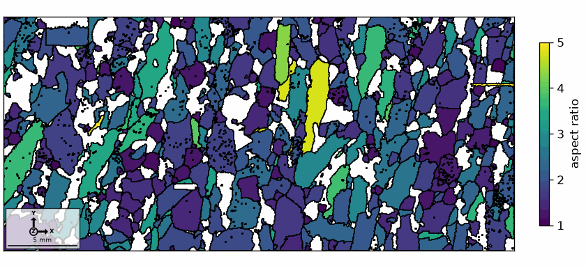
Elongated grains appear at the high end of the colour range, whereas nearly equiaxed grains appear near one. Values above five share the top colour because setColorRange([1, 5]) clips the displayed range.

Check the length yourself

MATLAB does not verify that a newly assigned property has the correct length: a property that is too short is accepted silently and fails only when later indexing requests an entry that does not exist. The port checks the length on assignment, so the mistake stops where it is made.

try:
  grains.nonsense = [1, 2, 3]
except ValueError as e:
  print(e)

the property 'nonsense' has 3 entries, the grains 3185

How properties are implemented

The dynProp mechanism implements the prop structure and the overloaded indexing, concatenation, and subsetting used here. Classes such as EBSD and grain2d share it, so a new property automatically participates in those operations.

Import interfaces use the same mechanism. Every column of an .ang or .ctf file that MTEX does not recognise as position, phase, or orientation becomes a property.

References

This page documents MTEX’s per-element storage mechanism and does not rely on an external method or definition.

Next

Glossary gives concise definitions of the data types and conventions used throughout MTEX documentation.

@article{bachmann2010mtex,
  author  = {F. Bachmann and R. Hielscher and H. Schaeben},
  title   = {Texture Analysis with MTEX - Free and Open Source Software Toolbox},
  journal = {Solid State Phenomena},
  volume  = {160},
  pages   = {63-68},
  year    = {2010},
  doi     = {10.4028/www.scientific.net/SSP.160.63},
  url     = {https://doi.org/10.4028/www.scientific.net/SSP.160.63}
}