Options

An MTEX command first receives the arguments it needs to do its job. Optional keyword arguments then adjust how that job is done. A flag is an option whose value is True or False and switches a behaviour on or off.

In the following pattern, data is a required argument, resolution is an option name, and 5*degree is its value. The final contour=True is a flag.

command(data, resolution=5*degree, contour=True)

Options are always optional, may be given in any order, and follow the required arguments. This lets you begin with a default call and add only the controls that matter for the result you need. The names are MTEX’s: MATLAB’s 'resolution',5*degree is resolution=5*degree here, and MATLAB’s flag 'contour' is contour=True.

A plotting option in practice

MTEX plotting commands understand the resolution option. It specifies how finely a continuous function is evaluated before it is drawn. A large angular step makes a coarse evaluation grid; a small step makes a fine grid and takes more time.

Compare pole figures of the same orientation density function (ODF), first on a 10 degree grid and then on a 2.5 degree grid. An ODF describes how frequently orientations occur in a material.

from mtex import *

odf = SantaFe()
h = Miller(1, 0, 0, odf.CS)

newMtexFigure(layout=[1, 2])
plotPF(odf, h, resolution=10 * degree, contour=True, lineWidth=2)
nextAxis()
plotPF(odf, h, resolution=2.5 * degree, contour=True, lineWidth=2)

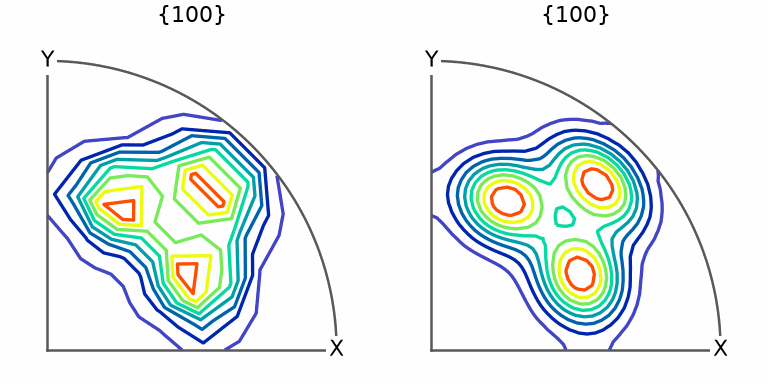
Both plots show the same three maxima. On the left, the 10 degree contour lines are visibly polygonal because the evaluation grid appears as kinks. On the right, the 2.5 degree contour lines are smooth curves. The resolution determines whether the drawing is limited by the function or by the grid on which MTEX evaluated it.

The default resolution is a compromise between detail and run time. Use a finer resolution when a figure will be published or when the grid is visible in a curve that should be smooth.

Flags

A flag takes the value True. The contour=True flag above asks for contour lines instead of a smooth colour plot. Flags and other options may be mixed freely and given in any order.

Python refuses the same keyword twice in one call. A wrapper that passes on its **kwargs and still overrides one of its own defaults merges the two dictionaries, the later value winning, as MATLAB’s rule for a repeated option does:

def myPlot(odf, h, **kwargs):
  return plotPF(odf, h, **{'contour': True, **kwargs})

Two traps

A misspelt option is not always caught. A command with a fixed set of options, such as calcGrains, refuses an unknown name: calcGrains(ebsd, theshold=10*degree) raises TypeError: calcGrains() got an unexpected keyword argument 'theshold'. The plotting commands, however, read the options they know and pass the rest on to matplotlib, which ignores what it does not use, so a misspelt plotting option runs and quietly uses the default. In MATLAB every command ignores an unknown option; the exact typo above survived for years in a published tutorial because the default happened to be the intended value. Copy option names rather than typing them.

Options are matched by their exact spelling. The plotting commands accept MATLAB’s capitalised spellings of the common options as well, lineWidth beside linewidth, but colourRange is not an option at all.

Finding the accepted names

Each MTEX command lists the options and flags it understands in its own help. For example, the help for calcGrains shows its signature with every keyword:

help(calcGrains)

Start with the command’s default call, inspect its help, and then append the documented names. This workflow avoids silent spelling errors and makes each non-default choice visible in the script.

References

This page documents MTEX’s calling convention and does not rely on an external method or definition.

Next

Properties explains the named values stored inside MTEX objects and how those values differ from the options passed to a command.

@article{bachmann2010mtex,
  author  = {F. Bachmann and R. Hielscher and H. Schaeben},
  title   = {Texture Analysis with MTEX - Free and Open Source Software Toolbox},
  journal = {Solid State Phenomena},
  volume  = {160},
  pages   = {63-68},
  year    = {2010},
  doi     = {10.4028/www.scientific.net/SSP.160.63},
  url     = {https://doi.org/10.4028/www.scientific.net/SSP.160.63}
}