Spatial Transforms

A spatial transform maps positions in one coordinate system to positions in another. It can describe the distortion between an EBSD map and an SEM image, stage drift during a scan, or the foreshortening of a tilted surface.

This is different from a reference frame, the coordinate system in which specimen or crystal data are expressed. A spatial transform moves map positions but does not correct the orientations stored at those positions. Use Reference Frame Alignment when the map coordinates and Euler angles do not refer to the same specimen frame.

A function can move positions too. A spatialTransform also composes, inverts, displays itself, fits measured point pairs, and can be stored for another data set. Maps and Images explains how two images first come to share a specimen coordinate system and array layout.

import numpy as np

from mtex import *

plottingConvention.default('y↑→x')
ebsd = mtexdata('twins')

Direction Is the Contract

One rule fixes everything else: T maps a position in coordinate system A to the position of the same physical point in coordinate system B.

The product T2 * T1 reads in matrix order, so T1 is applied first. Filling a regular output grid uses inv(T) rather than T. For each target pixel, the resampler has to ask where it came from, not where it goes.

Spatial transforms are two dimensional. They act on \(x\) and \(y\) and leave \(z\) unchanged.

T = spatialTransformRigid(vector3d(5, -2, 0))
T

spatialTransformRigid
  model  stage  parameters
  rigid  ·      move (5, -2)

Apply a transform to positions with *, or call eval explicitly.

pos = ebsd.pos[0, 0:3]
posMoved = T * pos

np.column_stack([pos.x.ravel(), posMoved.x.ravel()])

array([[0. , 5. ],
       [0.3, 5.3],
       [0.6, 5.6]])

Choose the Smallest Model That Describes the Distortion

Each class represents a different amount and pattern of spatial freedom. The names are historical, so read their meanings rather than guessing from them:

• spatialTransformId means that nothing separates the two coordinate systems.
• spatialTransformRigid is one translation, the same everywhere. It does not include a rotation.
• spatialTransformShift is a full 2D affine map: translation, rotation, scale, and shear in one homogeneous matrix.
• spatialTransformProjective is a homography. It keeps lines straight, but parallel lines need not remain parallel, as in a perspective view of a tilted plane.
• spatialTransformTilt is the staged model used to recover specimen tilt from repeatedly correlated image pairs.
• spatialTransformPoly describes a displacement that varies polynomially across the coordinate system.
• spatialTransformDrift varies only along the slow scan direction. It models rolling-shutter-like scan drift rather than an arbitrary smooth field.
• spatialTransformField stores measured displacements and interpolates between their positions without imposing a parametric model.
• spatialTransformHandle wraps a function when none of the fitted models applies.

Start with the least flexible model that has a physical reason to be present. A flexible model can follow noise and may extrapolate badly beyond the point pairs. Correspondences should span the area that will be transformed, and residuals should also be checked at withheld landmarks.

Differently modelled hops can be stored in one list. Such a list is an ordered sequence of hops, not a set of alternatives. It is primarily a container: combine the required hops or process them one at a time before calling methods such as inv on them.

hops = [spatialTransformRigid(vector3d(1, 0, 0)), spatialTransformPoly(np.zeros((3, 2)), 1)]
for hop in hops:
  print(hop)

spatialTransformRigid
  model  stage  parameters
  rigid  ·      move (1, 0)
spatialTransformPoly
  model   stage  parameters
  poly11  ·      |c| = 0

Fit a Transform From Two Point Sets

A transform is usually measured rather than written down. Locate the same features in both coordinate systems, then ask the chosen class for the member of its family that maps the first set onto the second. The two sets must use the same length unit and point order.

The geometric minimum is not enough for a reliable fit. An affine needs at least three non-collinear pairs, a homography at least four well-spread pairs, and a degree-two polynomial at least six. More pairs let a fit expose noise and mismatches.

For an example with a known answer, apply a projective distortion to map positions and fit the homography back from the resulting pairs.

T0 = spatialTransformProjective([[1, 0.02, 3], [-0.01, 1.05, -2], [1e-4, 2e-4, 1]])

posA = ebsd.pos.flatten()[::50]
posB = T0 * posA

T = spatialTransformProjective.fit(posA, posB)
T

spatialTransformProjective
  model       stage  parameters
  projective  ·      perspective (0.0001, 0.0002)

The maximum error is at rounding level.

np.max(norm(T * posA - posB))

2.5619e-14

Real correspondences are not this clean. Projective and polynomial fits use Tukey bisquare reweighting, so points that disagree with the consensus lose influence. Here every tenth target point is moved somewhere else.

posBad = posB.copy()
posBad[::10] = posBad[::10] + vector3d(30, -40, 0)

TBad = spatialTransformProjective.fit(posA, posBad)

np.max(norm(TBad * posA - posB))

7.1409e-14

The homography is fitted after both point sets are centred and scaled to a common spread, Hartley’s normalisation. Without it the algebraic residual of the fit weighs a point by its distance from the origin, and which tenth of the points is spoiled then decides whether the reweighting finds the transform.

Other classes match their physical model: a rigid fit takes a weighted mean displacement, an affine uses weighted least squares, drift uses a median displacement per scan line, and a field keeps the samples exactly.

Where a confidence per pair is available, pass it with weights= instead of asking the fit to infer every bad match. Cross-correlation supplies such weights.

Declare a Model With + and Compose Fitted Transforms With *

There are two ways to put transforms together, and they are not the same operation.

* composes fitted transforms and simplifies where it can. It decides by value, so an operand that reports isid disappears. An unfitted prototype has zero coefficients and therefore reports itself as the identity. In the product below, the shift silently disappears and only the drift remains.

spatialTransformShift() * spatialTransformDrift()

spatialTransformDrift
  model  stage  parameters
  drift  ·      (no knots)

+ declares a model. It reads left to right in the order the stages are applied and keeps both. Only a literal spatialTransformId is dropped, because that class means that nothing separates the two coordinate systems.

spatialTransformShift() + spatialTransformDrift()

spatialTransformComposite
  model        stage  parameters
  shift-drift  shift  scale 1 × 1, rotate 0°, shear 0°, move (0, 0)
               drift  (no knots)

Use + for a distortion model that is about to be fitted, and * for transforms whose coefficients are already known. Here + chains maps; it does not add displacements as + on a vector3d would.

Both operations flatten composites rather than nesting them, and their application order is consistent.

R = spatialTransformRigid(vector3d(1, -2, 0))
S = spatialTransformShift([[1, 0.1, 0], [0, 1, 0], [0, 0, 1]])

np.max(norm((R + S) * posA - S * (R * posA)))

0

Inverting

Rigid, affine, projective, and degree-one polynomial transforms have exact inverses. Their inv returns another closed-form transform.

inv(T)

spatialTransformProjective
  model       stage  parameters
  projective  ·      perspective (-0.000102, -0.000189)

A degree-two polynomial, drift spline, or scattered field has no general closed-form inverse. Its inverse is a spatialTransformInverse, which solves for each source position iteratively.

P = spatialTransformPoly.fit(posA, posB, degree=2)

Pinv = inv(P)
Pinv

spatialTransformInverse
  model       stage  parameters
  inv-poly22  ·      |c| = 3.606

The round trip returns the sampled positions to rounding level.

np.max(norm(Pinv.eval(P * posA) - posA))

6.5249e-11

Iteration converges while the displacement gradient remains below one in the queried region. A field that folds has no unique inverse. Asking far outside the region used for fitting can also fail, and the inverse reports either failure rather than returning a wrong position.

Collapse a Chain at Chosen Positions

Evaluating every stage repeatedly is wasted work when the chain will be applied to many pixels. discretize samples a chain at chosen positions and returns one spatialTransformField.

F = discretize(R + S, posA)
F

spatialTransformField
  model  stage  parameters
  field  ·      458 points, |u| <= 5.274

The field agrees with the chain at the sample positions. Between them it interpolates linearly over the triangulation of the samples, and beyond them it takes the nearest sample, so the sampling density controls fidelity.

np.max(norm(F * posA - (R + S) * posA))

8.8818e-16

Apply a Transform to an EBSD Map

transform moves every pixel and carries its unit cell with it. Orientations, phase labels, and all per-pixel properties remain untouched. A spatial transform therefore corrects map geometry, not an orientation or specimen-reference-frame error.

Carrying the unit cell is exact for an affine transform. For a nonlinear transform, one global unit cell can only represent the local transform at the map centre. The second argument may be a spatialTransform or a plain function.

ebsdT = transform(ebsd, S)

newMtexFigure(layout=[1, 2])
plot(ebsd, ebsd.bc, micronbar=False)
mtexColorMap('gray')
mtexTitle('as imported')
nextAxis()
plot(ebsdT, ebsdT.bc, micronbar=False)
mtexColorMap('gray')
mtexTitle('sheared')

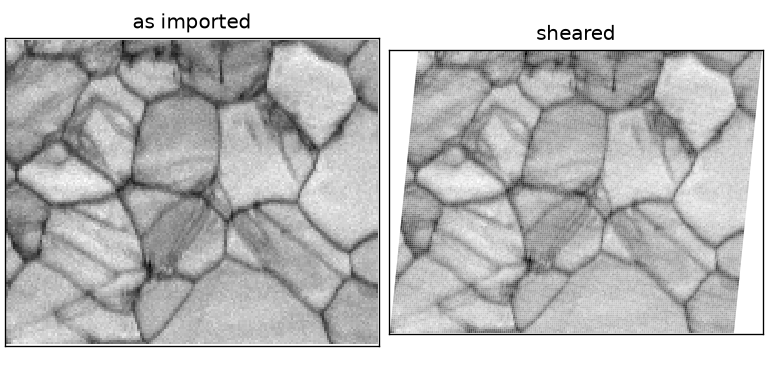
The right map has a sheared footprint, while the band-contrast values keep the same spatial order. The transform changed geometry, not the property.

Because this affine transform has an exact inverse, the original pixel positions are recovered.

ebsdBack = transform(ebsdT, inv(S))
np.max(norm(ebsdBack.pos - ebsd.pos))

7.1054e-15

Where the Point Pairs Come From

Nothing above measured a distortion: posA and posB were manufactured. In practice, pairs often come from correlating two images of the same area. xcfShift divides their shared region into tiles, phase correlates each tile with its counterpart, and returns a displacement and correlation-peak height for every tile.

The images must first share a pixel grid, and their stored order must refer to the same specimen directions. With mapImage inputs, xcfShift returns positions and displacements in specimen units rather than pixels.

The peak height is a fit weight, not a registration diagnostic. A tile on featureless background must not receive an equal vote:

u, peak, pos = xcfShift(imRef, imTest)
T = spatialTransformShift.fit(pos, pos + u, weights=peak)

Maps and Images prepares that common geometry. TrueEBSD Distortion Correction runs the complete chain on real data and checks the residual after correction.

References

• G. Nolze, Image distortions in SEM and their influences on EBSD measurements, Ultramicroscopy 107, 172–183, 2007, relates specimen tilt, scan geometry, and orientation error.
• V. S. Tong and T. B. Britton, TrueEBSD: Correcting spatial distortions in electron backscatter diffraction maps, Ultramicroscopy 221, 113130, 2021, develops the physically staged correction used by TrueEBSD.
• M. Guizar-Sicairos, S. T. Thurman, and J. R. Fienup, Efficient subpixel image registration algorithms, Optics Letters 33, 156–158, 2008, gives the Fourier-domain subpixel registration method used by xcfShift.
• B. Zitova and J. Flusser, Image registration methods: a survey, Image and Vision Computing 21, 977–1000, 2003, organizes registration into feature detection, matching, transform choice, and resampling.
• R. Hartley and A. Zisserman, Multiple View Geometry in Computer Vision, second edition, Cambridge University Press, 2004, develops homogeneous coordinates, homographies, the direct linear transform and its normalisation.

Next

Continue with TrueEBSD Distortion Correction to fit a sequence of physical distortion models to real EBSD and SEM images. See Square and Hex Grids when the transformed map must recover or preserve its lattice structure.

Correct the geometry before grain reconstruction when grain shape, boundary length, or correlative overlap matters. If grains already exist, transform both the map and its grain map.

@article{bachmann2010mtex,
  author  = {F. Bachmann and R. Hielscher and H. Schaeben},
  title   = {Texture Analysis with MTEX - Free and Open Source Software Toolbox},
  journal = {Solid State Phenomena},
  volume  = {160},
  pages   = {63-68},
  year    = {2010},
  doi     = {10.4028/www.scientific.net/SSP.160.63},
  url     = {https://doi.org/10.4028/www.scientific.net/SSP.160.63}
}