
A kernel on the rotation group is a radially symmetric scalar function:
\[\widetilde\psi\colon\mathrm{SO}(3)\to\mathbb R.\]Radial symmetry means that the value depends only on the rotation angle \(\omega(R)\in[0,\pi]\), not on the rotation axis. With \(t=\cos(\omega(R)/2)\), MTEX writes
\[\widetilde\psi(R)=\psi(t).\]Kernels set the shape of localized peaks in orientation space. Read Unimodal ODF Shapes for a direct comparison of their halfwidths, profiles and pole-figure projections. This page explains the series representation and the constructor for every kernel family.
import matplotlib.pyplot as plt
import numpy as np

from mtex import *
One coefficient per harmonic degree
A general SO3FunHarmonic has \((2n+1)^2\) Fourier, Wigner-D or
C-coefficients at degree \(n\). Radial symmetry reduces this entire block to
one coefficient \(\widehat\psi_n\). MTEX uses the Chebyshev expansion
where \(\mathcal U_{2n}\) is the Chebyshev polynomial of the second kind
and degree \(2n\). An SO3Kernel stores the scaled coefficients
\(a_n=(2n+1)\widehat\psi_n\) in its A property.
A custom kernel can therefore be constructed directly from its \(a_n\). The following values are \(a_0=1\), \(a_1=0\), \(a_2=3\) and \(a_3=1\).
psi = SO3Kernel([1, 0, 3, 1])
psi
SO3Kernel
  bandwidth: 3
  halfwidth: 40°
plot(psi)
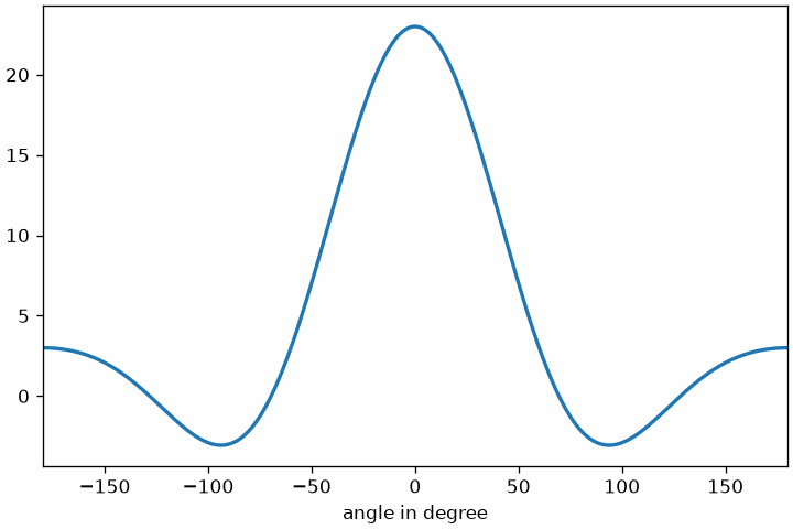
The oscillating curve is the Chebyshev series evaluated from \(-180^\circ\) to \(180^\circ\). Arbitrary coefficients need not define a nonnegative or normalized density.
From a kernel to a radial orientation function
An SO3FunRBF places a copy of a kernel at a
chosen centre orientation. Here a de la Vallee Poussin kernel with
\(20^\circ\) halfwidth produces one localized rotational function.
psi = SO3DeLaValleePoussinKernel(halfwidth=20 * degree)
psi
SO3DeLaValleePoussinKernel
  bandwidth: 13
  halfwidth: 20°
SO3F = SO3FunRBF(orientation.rand(rng=np.random.default_rng(1)), psi)
SO3F
SO3FunRBF (1 → y↓→x)
  unimodal component
    kernel: de la Vallee Poussin, halfwidth 20°
    center: 1 orientation
    weight: 1
    Bunge Euler angles in degree
    phi1   Phi  phi2  weight
     274  25.7   322       1
plot(SO3F)
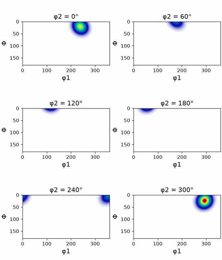
The sections show one peak about the sampled centre. The kernel controls
how its value falls with angular distance; the SO3FunRBF supplies the
centre and any symmetry-equivalent copies.
Pass a kernel to unimodalODF to choose the profile of
a model ODF. uniformODF uses a kernel internally to
represent its constant value, but does not require a kernel argument.
Kernels are also used when estimating an ODF from EBSD orientations.
Halfwidth and bandwidth answer different questions
The halfwidth is the angular distance at which the profile has fallen to half its maximum. It describes spread and is not normally a cutoff. The bandwidth is the largest stored harmonic degree. It describes spectral cost, not visible width.
Many constructors accept a halfwidth or bandwidth in addition to their native parameter, but support differs by family. This constructor chooses a \(30^\circ\) de la Vallee Poussin halfwidth.
psi = SO3DeLaValleePoussinKernel(halfwidth=30 * degree)
psi
SO3DeLaValleePoussinKernel
  bandwidth: 9
  halfwidth: 30°
plot(psi)
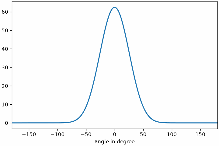
The curve crosses half its peak at \(30^\circ\). It remains positive beyond that angle, so the halfwidth should not be read as a hard boundary.
Choosing a family
The available families emphasize different properties:
` family main characteristic typical use ` |
` de la Vallee Poussin nonnegative and finite for integer $\kappa$ ODFs, misorientation distributions and pole figures ` |
` Dirichlet exact spectral cutoff with unit Fourier coefficients physical-property calculations ` |
` Abel–Poisson nonnegative with geometric spectral decay smooth radial peaks ` |
` von Mises–Fisher nonnegative exponential angular profile smooth radial peaks ` |
` Gauss–Weierstrass heat-kernel spectral decay smoothing by harmonic degree ` |
` Sobolev coefficients weighted by derivative order Sobolev operators rather than densities ` |
` Laplace inverse-power spectral decay inverse differential operators ` |
` squared singularity nonnegative rational singularity family alternative radial profile ` |
` bump constant inside a strict angular cutoff compact support ` |
The profile plot in each section answers what the kernel looks like in orientation space. The spectrum beside it shows \(\widehat\psi_n=a_n/(2n+1)\) and therefore its harmonic cost.
The de la Vallee Poussin kernel
For \(t\in[0,1]\), the de la Vallee Poussin kernel is
\[K(t)=\frac{B(\frac32,\frac12)} {B(\frac32,\kappa+\frac12)}t^{2\kappa},\]where \(B\) is the beta function. For positive integer \(\kappa\in\mathbb N\setminus\{0\}\) it has the finite expansion
\[\psi_\kappa(t)= \frac{(\kappa+1)2^{2\kappa-1}}{\binom{2\kappa-1}{\kappa}}t^{2\kappa} =\binom{2\kappa+1}{\kappa}^{-1} \sum_{n=0}^{\kappa}(2n+1)\binom{2\kappa+1}{\kappa-n} \mathcal U_{2n}(t).\]This family is recommended for texture analysis because it is positive in orientation space and, for integer \(\kappa\), has no Fourier truncation error. A requested halfwidth generally gives a noninteger \(\kappa\); MTEX then stores coefficients down to its numerical cutoff.
psi1 = SO3DeLaValleePoussinKernel(halfwidth=15 * degree)
psi1
SO3DeLaValleePoussinKernel
  bandwidth: 17
  halfwidth: 15°
psi2 = SO3DeLaValleePoussinKernel(halfwidth=20 * degree)
psi2
SO3DeLaValleePoussinKernel
  bandwidth: 13
  halfwidth: 20°
The corresponding parameters are \(\kappa=40.34\) and \(22.64\). Compare their profiles and spectra in one figure.
plt.figure()
plt.subplot(1, 2, 1)
plot(psi1, lineWidth=2)
hold(True)
plot(psi2, lineWidth=2)
hold(False)
plt.subplot(1, 2, 2)
plotSpectrum(psi1, lineWidth=2)
hold(True)
plotSpectrum(psi2, lineWidth=2)
hold(False)
legend('halfwidth = 15°', 'halfwidth = 20°')
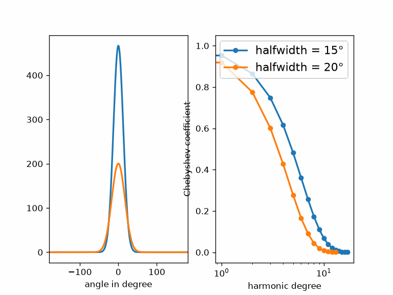
The \(15^\circ\) kernel is narrower and taller. Its coefficients persist to higher degrees, illustrating the cost of resolving a sharper peak.
The Dirichlet kernel
The Dirichlet kernel is the finite series
\[\psi_N(t)=\sum_{n=0}^{N}(2n+1)\mathcal U_{2n}(t).\]It integrates to one. Its Fourier coefficients equal one through bandwidth \(N\) and are zero above it. This exact cutoff is useful for calculating physical properties, although the orientation-space profile oscillates and can be negative.
psi1 = SO3DirichletKernel(10)
psi1
SO3DirichletKernel
  bandwidth: 10
  halfwidth: 13.1°
psi2 = SO3DirichletKernel(5)
psi2
SO3DirichletKernel
  bandwidth: 5
  halfwidth: 24.1°
plt.figure()
plt.subplot(1, 2, 1)
plot(psi1, lineWidth=2)
hold(True)
plot(psi2, lineWidth=2)
hold(False)
plt.subplot(1, 2, 2)
plotSpectrum(psi1, lineWidth=2)
hold(True)
plotSpectrum(psi2, lineWidth=2)
hold(False)
legend('bandwidth = 10', 'bandwidth = 5')
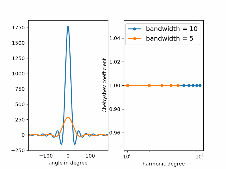
The bandwidth-10 profile has a sharper central lobe and more side lobes. The spectrum verifies that every retained Fourier coefficient is exactly one for both kernels.
The Abel–Poisson kernel
The nonnegative Abel–Poisson kernel uses \(\kappa\in(0,1)\) and the series
\[\psi_\kappa(t)=\sum_{n=0}^{\infty}(2n+1)\kappa^{2n} \mathcal U_{2n}(t).\]psi1 = SO3AbelPoissonKernel(halfwidth=15 * degree)
psi1
SO3AbelPoissonKernel
  bandwidth: 19
  halfwidth: 15°
psi2 = SO3AbelPoissonKernel(halfwidth=20 * degree)
psi2
SO3AbelPoissonKernel
  bandwidth: 15
  halfwidth: 20°
These halfwidths give \(\kappa=0.82\) and \(0.76\), respectively.
plt.figure()
plt.subplot(1, 2, 1)
plot(psi1, lineWidth=2)
hold(True)
plot(psi2, lineWidth=2)
hold(False)
plt.subplot(1, 2, 2)
plotSpectrum(psi1, lineWidth=2)
hold(True)
plotSpectrum(psi2, lineWidth=2)
hold(False)
legend('halfwidth = 15°', 'halfwidth = 20°')
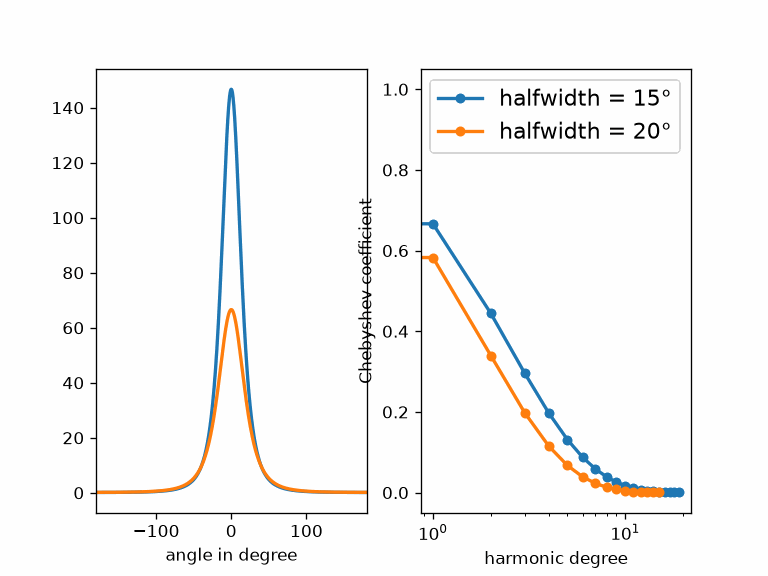
Both profiles remain nonnegative and have long tails. The narrower kernel has the larger \(\kappa\), so its geometrically decaying coefficients remain significant to higher degree.
The von Mises–Fisher kernel
For \(\kappa>0\), the von Mises–Fisher kernel has the series
\[\psi_\kappa(t)=\sum_{n=0}^{\infty} \frac{\mathcal I_n(\kappa)-\mathcal I_{n+1}(\kappa)} {\mathcal I_0(\kappa)-\mathcal I_1(\kappa)}\mathcal U_{2n}(t),\]and the direct angular form
\[\psi_\kappa\!\left(\cos\frac{\omega(R)}2\right)= \frac{\mathrm e^{\kappa\cos\omega(R)}} {\mathcal I_0(\kappa)-\mathcal I_1(\kappa)}.\]Here \(\mathcal I_n\) is the modified Bessel function of the first kind,
\[\mathcal I_n(\kappa)=\frac1\pi\int_0^\pi \mathrm e^{\kappa\cos\omega}\cos(n\omega)\,\mathrm d\omega.\]psi1 = SO3vonMisesFisherKernel(halfwidth=15 * degree)
psi1
SO3vonMisesFisherKernel
  bandwidth: 18
  halfwidth: 15°
psi2 = SO3vonMisesFisherKernel(halfwidth=20 * degree)
psi2
SO3vonMisesFisherKernel
  bandwidth: 14
  halfwidth: 20°
These halfwidths give \(\kappa=20.34\) and \(11.49\), respectively.
plt.figure()
plt.subplot(1, 2, 1)
plot(psi1, lineWidth=2)
hold(True)
plot(psi2, lineWidth=2)
hold(False)
plt.subplot(1, 2, 2)
plotSpectrum(psi1, lineWidth=2)
hold(True)
plotSpectrum(psi2, lineWidth=2)
hold(False)
legend('halfwidth = 15°', 'halfwidth = 20°')
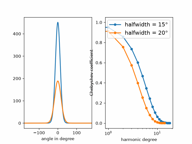
The exponential profiles are smooth and nonnegative. As before, the narrower peak requires appreciable coefficients at higher degrees.
The Gauss–Weierstrass kernel
The nonnegative Gauss–Weierstrass kernel uses \(\kappa>0\) and
\[\psi_\kappa(t)=\sum_{n=0}^{\infty}(2n+1) \mathrm e^{-n(n+1)\kappa}\mathcal U_{2n}(t).\]psi1 = SO3GaussWeierstrassKernel(0.025)
psi1
SO3GaussWeierstrassKernel
  bandwidth: 17
  halfwidth: 15.1°
psi2 = SO3GaussWeierstrassKernel(0.045)
psi2
SO3GaussWeierstrassKernel
  bandwidth: 13
  halfwidth: 20.3°
plt.figure()
plt.subplot(1, 2, 1)
plot(psi1, lineWidth=2)
hold(True)
plot(psi2, lineWidth=2)
hold(False)
plt.subplot(1, 2, 2)
plotSpectrum(psi1, lineWidth=2)
hold(True)
plotSpectrum(psi2, lineWidth=2)
hold(False)
legend('κ = 0.025 (15.14°)', 'κ = 0.045 (20.33°)')
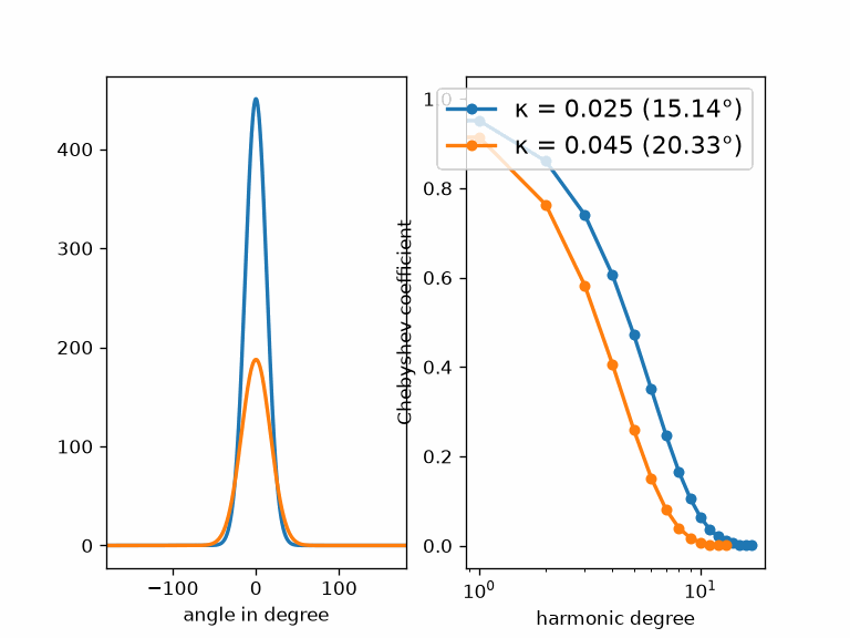
The measured halfwidths are \(15.14^\circ\) and \(20.33^\circ\), rather than exactly \(15^\circ\) and \(20^\circ\). Larger \(\kappa\) damps high degrees more strongly and therefore produces the broader profile.
The Sobolev kernel
A Sobolev kernel of order \(s\) and bandwidth \(N\) is
\[\psi_s(t)=\sum_{n=0}^{N}(2n+1)(n(n+1))^s \mathcal U_{2n}(t).\]The coefficient at \(n=0\) is zero. Positive \(s\) amplifies high harmonic degrees, so this family represents a differential weighting rather than a nonnegative density kernel.
psi1 = SO3SobolevKernel(1, bandwidth=15)
psi1
SO3SobolevKernel
  bandwidth: 15
  halfwidth: 8.12°
psi2 = SO3SobolevKernel(1.2, bandwidth=15)
psi2
SO3SobolevKernel
  bandwidth: 15
  halfwidth: 8.03°
plt.figure()
plt.subplot(1, 2, 1)
plot(psi1, lineWidth=2)
hold(True)
plot(psi2, lineWidth=2)
hold(False)
plt.subplot(1, 2, 2)
plotSpectrum(psi1, lineWidth=2)
hold(True)
plotSpectrum(psi2, lineWidth=2)
hold(False)
legend('s = 1', 's = 1.2')
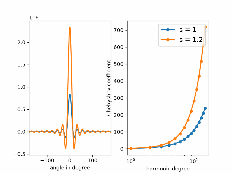
Both profiles oscillate because they are truncated at bandwidth 15. The spectrum for \(s=1.2\) rises faster, placing more weight on fine angular variation.
The Laplace kernel
The Laplace kernel sets its degree-zero coefficient to zero and uses
\[\psi(t)=\sum_{n=1}^{\infty} \frac{2n+1}{4n^2(2n+2)^2}\mathcal U_{2n}(t).\]psi = SO3LaplaceKernel()
psi
SO3LaplaceKernel
  bandwidth: 4
  halfwidth: 55.1°
plt.figure()
plt.subplot(1, 2, 1)
plot(psi, lineWidth=2)
plt.subplot(1, 2, 2)
plotSpectrum(psi, lineWidth=2)
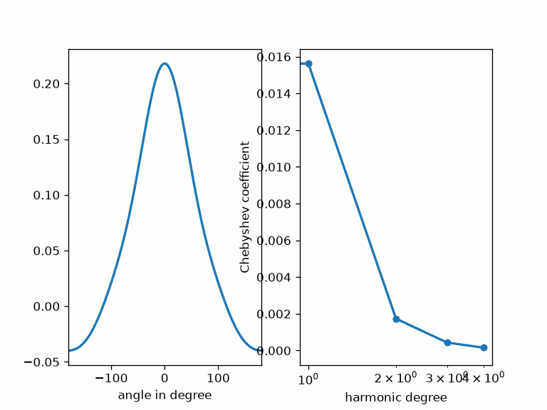
The profile is not a normalized density because its mean, the degree-zero coefficient, is zero. MTEX stores this kernel only to bandwidth 4, so the spectrum panel is four markers falling steeply and then stopping. The series itself continues past them with inverse-power decay.
The squared singularity kernel
The nonnegative squared singularity kernel depends on \(\kappa\in(0,1)\) and has the series
\[\psi_\kappa(t)=\sum_{n=0}^{\infty} \widehat f_n(\kappa)\mathcal U_{2n}(t).\]Its Chebyshev coefficients follow the three-term recursion
\[\widehat f_0=1,\] \[\widehat f_1=\frac{1+\kappa^2}{2\kappa} -\frac1{\log\frac{1+\kappa}{1-\kappa}},\] \[\widehat f_n= \frac{(2n-3)(2n+1)(1+\kappa^2)} {(2n-1)(n-1)2\kappa}\widehat f_{n-1}(\kappa) -\frac{2\kappa(n-2)(2n+1)}{2n-3}\widehat f_{n-2}(\kappa).\]psi1 = SO3SquareSingularityKernel(0.2)
psi1
SO3SquareSingularityKernel
  bandwidth: 5
  halfwidth: 77.5°
psi2 = SO3SquareSingularityKernel(0.3)
psi2
SO3SquareSingularityKernel
  bandwidth: 7
  halfwidth: 54.9°
plt.figure()
plt.subplot(1, 2, 1)
plot(psi1, lineWidth=2)
hold(True)
plot(psi2, lineWidth=2)
hold(False)
plt.subplot(1, 2, 2)
plotSpectrum(psi1, lineWidth=2)
hold(True)
plotSpectrum(psi2, lineWidth=2)
hold(False)
legend('κ = 0.2', 'κ = 0.3')
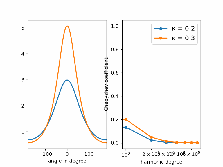
The two parameters change both the central concentration and the rate of spectral decay. Unlike the Dirichlet and Sobolev profiles, both curves remain nonnegative.
The bump kernel
The bump kernel depends on a radius \(r\in(0,\pi)\). It is constant inside that radius and exactly zero outside it. With
\[U_r=\{R\in\mathrm{SO}(3)\mid\lvert\omega(R)\rvert<r\},\]the normalized indicator is
\[\widetilde\psi_r(R)=\frac1{\lvert U_r\rvert} \mathbf 1_{\{R\in U_r\}}.\]The constant is chosen so that the mean on \(\mathrm{SO}(3)\) is one.
psi1 = SO3BumpKernel(30 * degree)
psi1
SO3BumpKernel
  bandwidth: 1024
  halfwidth: 30°
psi2 = SO3BumpKernel(40 * degree)
psi2
SO3BumpKernel
  bandwidth: 1024
  halfwidth: 40°
plt.figure()
plt.subplot(1, 2, 1)
plot(psi1, lineWidth=2)
hold(True)
plot(psi2, lineWidth=2)
hold(False)
plt.subplot(1, 2, 2)
plotSpectrum(psi1, lineWidth=2)
hold(True)
plotSpectrum(psi2, lineWidth=2)
hold(False)
legend('halfwidth = 30°', 'halfwidth = 40°')
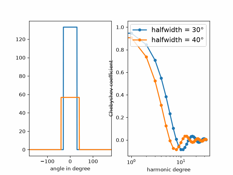
The flat tops and abrupt cutoffs distinguish the bump kernels from every smooth family above. Representing that discontinuity requires many Chebyshev coefficients; both objects store bandwidth 1024. This can lead to high runtimes even though the real-space definition is simple.
References
- H. Schaeben,
<https://doi.org/10.1155/TSM.33.365 The de la Vallee Poussin Standard Orientation Density Function>, Textures and Microstructures 33 (1999), 365–373, relates kernel halfwidth to the finite harmonic representation used for texture analysis.
- R. Hielscher,
<https://doi.org/10.1016/j.jmva.2013.03.014 Kernel density estimation on the rotation group and its application to crystallographic texture analysis>, Journal of Multivariate Analysis 119 (2013), 119–143, compares kernel families on \(\mathrm{SO}(3)\) and develops their use in crystallographic density estimation.
Next
Continue with Wigner-D Functions to see the harmonic basis whose radial coefficient blocks collapse to the single coefficient per degree used on this page.
Citing this page.
This page is part of the documentation of
MTEX, a free and open
source MATLAB toolbox for analyzing and modeling crystallographic textures.
It was written by The MTEX Developers and is published at
https://mtex-toolbox.github.io/SO3Kernels_py.html.
If you use MTEX, or reuse text or figures from this page, in your research,
please cite
F. Bachmann, R. Hielscher, H. Schaeben: Texture Analysis with MTEX - Free and Open Source Software Toolbox, Solid State Phenomena 160 (2010), 63-68. 10.4028/www.scientific.net/SSP.160.63
BibTeX
@article{bachmann2010mtex,
  author  = {F. Bachmann and R. Hielscher and H. Schaeben},
  title   = {Texture Analysis with MTEX - Free and Open Source Software Toolbox},
  journal = {Solid State Phenomena},
  volume  = {160},
  pages   = {63-68},
  year    = {2010},
  doi     = {10.4028/www.scientific.net/SSP.160.63},
  url     = {https://doi.org/10.4028/www.scientific.net/SSP.160.63}
}
Other papers describing specific MTEX methods are listed under Publications — please cite the one that best fits your application. The MTEX source code is licensed under the GNU General Public License v2.0; the text and figures of this documentation are licensed under CC BY 4.0, which permits reuse — including by automated systems — provided The MTEX Developers and this page are credited.