Wigner-D functions

Wigner-D functions play the role of sine and cosine waves for rotations. Weighted sums of them can represent any square-integrable function on the rotation group \(\mathrm{SO}(3)\).

Each function has a non-negative degree \(n\) and two orders \(k\) and \(l\), both between \(-n\) and \(n\). The command WignerD evaluates a complete matrix of orders at once.

Evaluate one degree

A real number passed to WignerD is the second Euler angle \(\beta\). The result below contains all Wigner-d functions of degree one at \(\beta=90\) degrees.

import matplotlib.pyplot as plt
import numpy as np

from mtex import *

beta = 90 * degree
d = WignerD(beta, 1)
d

array([[ 0.5   , -0.7071, -0.5   ],
       [ 0.7071,  0.    ,  0.7071],
       [-0.5   , -0.7071,  0.5   ]])

The rows and columns correspond to \(k=-1,0,1\) and \(l=-1,0,1\), respectively. In particular, the central value is zero at 90 degrees, while the corner values have magnitude \(0.5\).

Passing a rotation instead evaluates the generally complex Wigner-D functions. The normalize flag selects MTEX’s \(L_2\) normalization.

R = rotation.byEuler(20 * degree, 40 * degree, 10 * degree)
W = WignerD(R, 1, normalize=True)
W

array([[1.3245+0.7647j, 0.1367-0.7753j, 0.1995-0.0352j],
       [0.2693-0.7398j, 1.3268+0.j    , 0.2693+0.7398j],
       [0.1995+0.0352j, 0.1367+0.7753j, 1.3245-0.7647j]])

Follow the Wigner-d curves

The Wigner-d functions are ordinary functions of the single angle \(\beta\), so they can be drawn directly. Here are three entries from the degree-one matrix.

beta = np.linspace(0, np.pi, 181)
d = np.zeros((beta.size, 3))
for j in range(beta.size):
  Dj = WignerD(beta[j], 1)
  d[j] = [Dj[0, 0], Dj[1, 1], Dj[0, 2]]

plt.figure()
plt.plot(beta / degree, d, linewidth=2)
plt.xlim(0, 180)
plt.xlabel('beta in degree')
legend('$d^1_{-1,-1}$', '$d^1_{0,0}$', '$d^1_{-1,1}$', location='best')

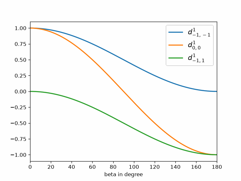
The first curve decreases from 1 to 0. The central curve crosses zero at 90 degrees, while the corner entry decreases from 0 to -1. These smooth shapes arise because the functions are polynomials in \(\cos(\beta/2)\) and \(\sin(\beta/2)\). Series in Wigner-d functions therefore converge quickly for smooth functions.

Build one basis function

The Wigner-D functions form an orthonormal basis of \(L_2(\mathrm{SO}(3))\). MTEX stores a weighted series in this basis as an SO3FunHarmonic object.

Its coefficient vector starts with the degree-zero block. The next nine entries are the degree-one matrix, stored one column at a time. The vector below therefore selects \(D_1^{1,-1}\).

F = SO3FunHarmonic([0, 0, 0, 1])
seriesValue = F.eval(R)
seriesValue

(0.19953333233923354+0.0351831100420756j)

The selected coefficient is row 3 and column 1 of the normalized matrix W above, W[2, 0] counted from zero. Both evaluations give approximately 0.1995 + 0.0352i.

directValue = W[2, 0]
directValue

(0.19953333233923354+0.035183110042075603j)

comparisonError = abs(seriesValue - directValue)
comparisonError

6.9389e-18

Normalization

Several normalizations of Wigner-D functions occur in the literature. MTEX defines the \(L_2\) norm by

With this measure, the constant function \(f=1\) has norm 1. Every normalized Wigner-D function also has \(\|D_n^{k,l}\|_2=1\).

norm(F)

1

The section Integration and Norms explains integration and norms for rotational functions in more detail.

The maths behind Wigner-D functions

In the Matthies ZYZ convention, write a rotation as \(\mathbf{R}=\mathbf{R}(\alpha,\beta,\gamma)\). MTEX defines the \(L_2\)-normalized Wigner-D function by

The real-valued Wigner-d function \(d_n^{k,l}\colon[0,\pi]\to\mathbb{R}\) is defined through the Jacobi polynomial \(P_s^{a,b}\) by

How the MTEX convention differs

MTEX’s definition differs slightly from other common definitions. It is compatible with the spherical harmonics, which form an orthonormal basis on the 2-sphere and are used to build harmonic spherical functions.

• The orders \(k\) and \(l\) are interchanged in the exponential factors compared with common definitions.
• The factor \(\sqrt{2n+1}\) gives each \(D_n^{k,l}\) unit \(L_2\) norm.
• The sign of \(d_n^{k,l}\) includes the contribution \(\min\{0,k\}+\min\{0,l\}\) through \((-1)^\nu\).
• MTEX parametrizes a Wigner-d function by the second Euler angle \(\beta\). Thus MTEX’s \(d_n^{k,l}(\beta)\) corresponds to \(d_n^{k,l}(x)\) with \(x=\cos(\beta)\) in definitions that use \(x\).

Composition and symmetry

For each degree \(n\), the Wigner-D functions are the matrix elements of a representation \(D_n\colon\mathrm{SO}(3)\to \mathbb{C}^{(2n+1)\mathbin{\times}(2n+1)}\). The representation is a group homomorphism. With MTEX’s order and normalization conventions,

and hence

Inversion exchanges the two orders and complex conjugates the value:

The Wigner-d functions also satisfy several useful symmetries:

References

• D. A. Varshalovich, A. N. Moskalev, and V. K. Khersonskii, Quantum Theory of Angular Momentum, World Scientific, 1988, gives common Wigner-D definitions against which MTEX’s order, sign, and normalization conventions can be compared.

Technical Details

WignerD and the coefficients fhat are MTEX’s; the port computes internally in the conventions of docs/design/harmonics.md and converts at the boundary. MATLAB’s 'normalize' flag is normalize=True, and a NumPy matrix is indexed from zero.

@article{bachmann2010mtex,
  author  = {F. Bachmann and R. Hielscher and H. Schaeben},
  title   = {Texture Analysis with MTEX - Free and Open Source Software Toolbox},
  journal = {Solid State Phenomena},
  volume  = {160},
  pages   = {63-68},
  year    = {2010},
  doi     = {10.4028/www.scientific.net/SSP.160.63},
  url     = {https://doi.org/10.4028/www.scientific.net/SSP.160.63}
}