Operations on Orientation-Dependent Functions

The common SO3Fun interface lets you calculate with functions much as NumPy calculates with arrays. This page starts from two functions and uses them for arithmetic, extrema, integration, differentiation and rotation. See Defining Orientation-Dependent Functions first if the representations are unfamiliar.

Two Example Functions

The first function is the Dubna ODF determined from neutron diffraction data. An ODF is an orientation density function.

import numpy as np

from mtex import *

plottingConvention.default('y↑→x')
SO3F1 = SO3Fun.dubna()
SO3F1

SO3FunRBF (Quartz → y↑→x)
  multimodal components
    kernel: de la Vallee Poussin, halfwidth 5°
    center: 20040 orientations
    weight: 1
    Bunge Euler angles in degree
    phi1   Phi  phi2    weight
      90  2.49   210   3.2e-06
      90  2.49   215  4.22e-06
      90  2.49   220  5.37e-06
      90  2.49   225  5.75e-06
      90  2.49   230   5.4e-06
       ⋮     ⋮     ⋮         ⋮
     7.5  97.1   7.5  1.58e-06
    52.5  97.1   292  1.21e-05
    57.5  97.1   298  8.61e-06
    62.5  97.1   302   6.1e-06
    67.5  97.1   308  5.68e-06

plot(SO3F1, 'sigma', sections=4)
mtexColorbar()

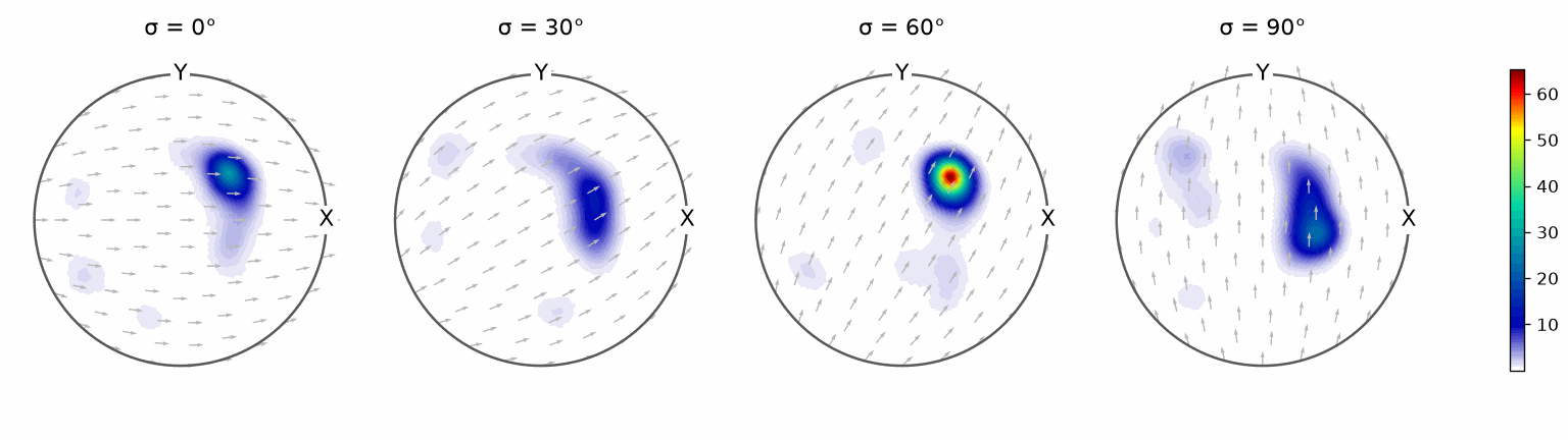
The unequal colours show that the measured orientations are not uniformly distributed. Several maxima appear across the sigma sections rather than one isolated ideal component.

The second function is a unimodal ODF. It places one radial kernel at the orientation R.

R = orientation.byAxisAngle(vector3d.Y, np.pi / 4, SO3F1.CS)
SO3F2 = SO3FunRBF(R, SO3DeLaValleePoussinKernel())
SO3F2

SO3FunRBF (Quartz → y↑→x)
  unimodal component
    kernel: de la Vallee Poussin, halfwidth 10°
    center: 1 orientation
    weight: 1
    Bunge Euler angles in degree
    phi1  Phi  phi2  weight
      90   45   270       1

plot(SO3F2, 'sigma', sections=4)
mtexColorbar()

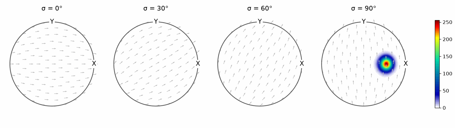
In contrast to the measured ODF, this plot contains one concentrated component. Its appearance in neighbouring sections is the cross-section of one three-dimensional peak in orientation space.

Arithmetic

Adding functions or scaling them produces another SO3Fun. MTEX can combine different internal representations in the same expression.

combined = 2 * SO3F1 + SO3F2
shiftedCombined = 1 + combined
shiftedCombined

SO3FunComposition (Quartz → y↑→x)
  components: 3
  SO3FunRBF (Quartz → y↑→x)
    multimodal components
      kernel: de la Vallee Poussin, halfwidth 5°
      center: 20040 orientations
      weight: 2
      Bunge Euler angles in degree
      phi1   Phi  phi2    weight
        90  2.49   210  6.41e-06
        90  2.49   215  8.44e-06
        90  2.49   220  1.07e-05
        90  2.49   225  1.15e-05
        90  2.49   230  1.08e-05
         ⋮     ⋮     ⋮         ⋮
⋮
    unimodal component
      kernel: de la Vallee Poussin, halfwidth 10°
      center: 1 orientation
      weight: 1
      Bunge Euler angles in degree
      phi1  Phi  phi2  weight
        90   45   270       1
  SO3FunRBF (Quartz → y↑→x)
    uniform component
      weight: 1

plot(combined, 'sigma', sections=4)
mtexColorbar()

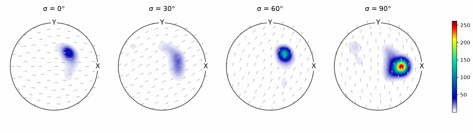
The combined plot retains features of the measured ODF and adds the narrow component from SO3F2. The constant in shiftedCombined raises every value equally, so it does not change the positions of those features.

Basic overloaded operations include -, scalar *, scalar /, pointwise *, pointwise / and pointwise **. Pointwise abs, sqrt, conj, exp and log also return functions.

Pointwise Minimum and Maximum

With two function arguments, max and min compare values independently at every orientation.

pointwiseMax = max(2 * SO3F1, SO3F2)
plot(pointwiseMax, 'sigma', sections=4)
mtexColorbar()

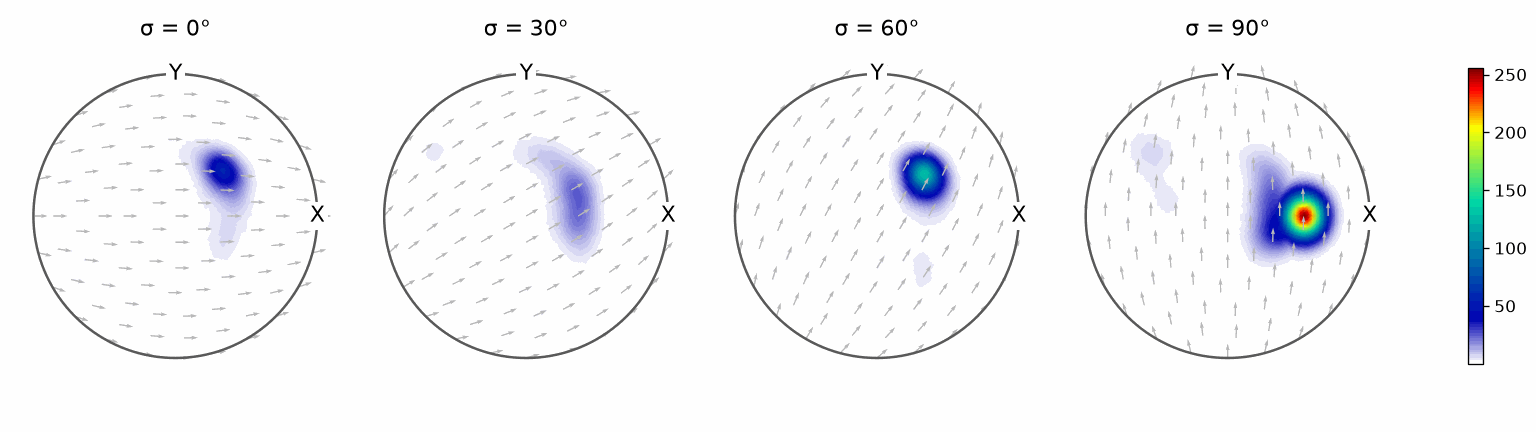
At every plotted orientation, the colour comes from whichever input has the larger value. The narrow peak survives where it rises above the doubled measured ODF.

pointwiseMin = min(2 * SO3F1, SO3F2)
plot(pointwiseMin, 'sigma', sections=4)
mtexColorbar()

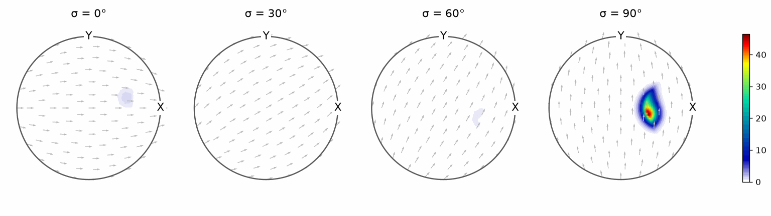
The minimum keeps the lower input instead. It clips each function wherever the other lies below it. Passing one function and one scalar performs the same comparison against a constant threshold.

Inverting the Argument

The inv operation composes a function with inversion. If g = inv(f), then the value of g at a rotation is the value of f at the inverse rotation.

The check below uses the harmonic representation of the Dubna ODF.

SO3F1Harmonic = SO3FunHarmonic(SO3F1, bandwidth=16)
g = inv(SO3F1Harmonic)

testRot = rotation(R)
valueAtR = SO3F1Harmonic.eval(testRot)
valueAtR

3.3518

inverseValue = g.eval(inv(testRot))
inverseValue

3.3518

The two displayed values agree, which checks the relation $g(\mathbf{R}^{-1}) = f(\mathbf{R})$ for this orientation.

Global and Local Extrema

The number and type of arguments change what min and max return.

• With one SO3Fun, they return its global extremum and its position.
• With two functions, they return the pointwise minimum or maximum function shown above.
• With one function and one scalar, they return a pointwise clipped function.
• With numLocal=n, they return up to n distinct local extrema and their positions.

The following search asks for the two largest local maxima of combined.

plot(combined, 'phi2', np.arange(4) * 30 * degree)
mtexColorbar()

maxValue, maxNodes = max(combined, numLocal=2)
annotate(maxNodes)

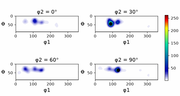
maxValue

array([262.0311, 188.8086])

maxNodes

orientation (Quartz → y↑→x)
  size: 2
  Bunge Euler angles in degree
  phi1   Phi  phi2
  89.7  44.5   270
   133  35.7   205

The annotations mark the two returned orientations. The first value is the global maximum, while the second is the next distinct local maximum.

Integration and Norms

mean returns the normalized integral over \(SO(3)\). It assigns the constant function one an integral of one. sum uses the full rotation-group volume \(8\pi^2\).

normalizedIntegral = mean(SO3F1)
normalizedIntegral

1.0000

integralFromSum = sum(SO3F1) / (8 * np.pi ** 2)
integralFromSum

1.0000

These two values agree because dividing sum by \(8\pi^2\) gives the same normalization as mean.

With this normalized measure, the \(L^2\) norm of a function is

It can be assembled from pointwise operations and mean.

normFromDefinition = sqrt(mean(abs(SO3F1) ** 2))
normFromDefinition

4.0425

The dedicated norm command computes the same quantity more efficiently. A small difference between the displayed results comes from the numerical approximations used by the two routes.

directNorm = norm(SO3F1)
directNorm

4.0425

Differentiation at One Orientation

The gradient at a particular orientation belongs to the tangent space of \(SO(3)\) at that orientation. MTEX represents it by an SO3TangentVector.

gradientAtR = grad(SO3F1, R)
gradientAtR

SO3TangentVector (left, y↑→x)
  reference: orientation (Quartz → y↑→x)
     x      y      z
  15.7  -45.5  -4.84

Roughly speaking, this tangent vector points in the direction of steepest ascent. Following it through the exponential map produces a new rotation. See Tangent Space Representation on SO(3) for that construction.

The Gradient Field

Without an evaluation orientation, grad returns the gradients at all orientations as an SO3VectorFieldHarmonic.

G = grad(SO3F1)
G

SO3VectorFieldHarmonic (Quartz → y↑→x)
  tangent space: left
  bandwidth    : 48

plot(SO3F1, 'sigma', sections=4)
hold(True)
plot(G, color='black', lineWidth=1, resolution=5 * degree)
hold(False)

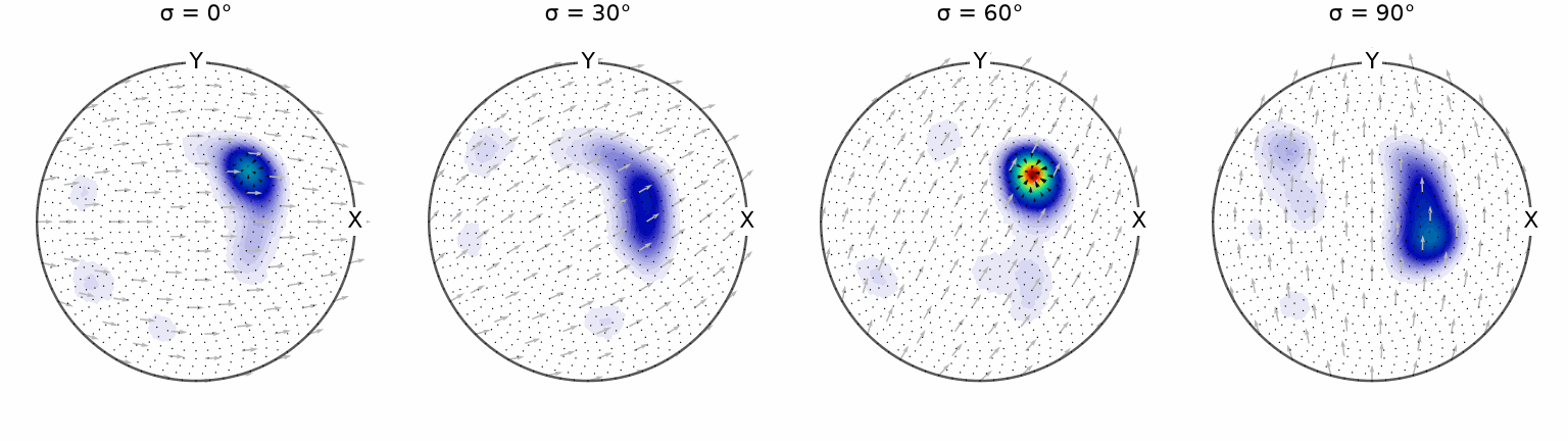
The section plot lays down a grey arrow field of its own, and the gradient is drawn in black on top of it. Read the black arrows. They are long where the ODF intensity changes quickly and almost invisible where it is nearly constant, and each points along the local direction of steepest ascent represented in that section.

Rotating a Function

rotate moves an orientation-dependent function by a specified rotation. This changes where its features occur. It is not a frame change, which would re-express the same physical function in a different reference frame.

rot = rotation.byEuler(30 * degree, 0 * degree, 90 * degree, 'Bunge')
rotated = rotate(SO3FunHarmonic(combined), rot)
rotated

SO3FunHarmonic (Quartz → y↑→x)
  bandwidth: 48
  mean     : 3

plot(rotated, 'sigma', sections=4)
mtexColorbar()

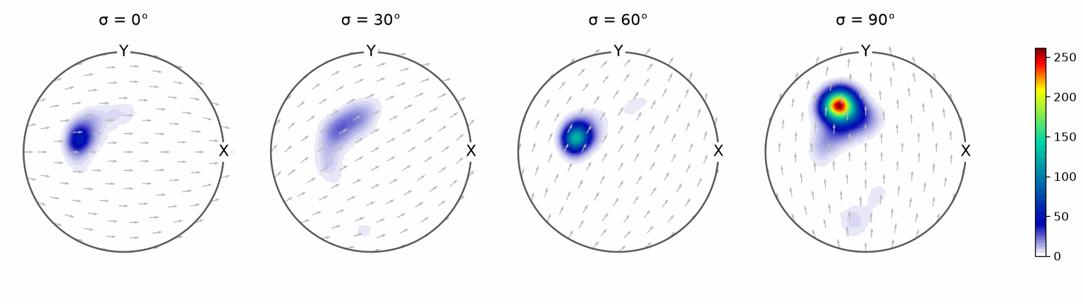
Compared with the earlier plot of combined, the same pattern is shifted through orientation space. Its amplitudes and internal arrangement are preserved by the rotation.

References

• H.-J. Bunge, Texture Analysis in Materials Science: Mathematical Methods, Butterworths, 1982, gives the orientation-space integration and ODF normalization used here.

Next

Continue with Plotting Orientation Functions to choose section types, projections and colour ranges for inspecting an SO3Fun.

Technical Details

MATLAB’s SO3Fun.dubna is an ODF stored with its specimen frame, whose plotting convention is y↓→x, so its plots have Y at the bottom although the page sets y↑→x; the port reconstructs the ODF from the pole figures, in the session’s frame, and draws Y at the top. The reconstruction differs in the digits: the two local maxima are 262.2 and 188.9 for MATLAB’s 262.2 and 187.9, the norm 4.032 for 4.027. MATLAB’s page says inv of the RBF form fails; the port’s inv works on every form, the page keeps MATLAB’s harmonic check.

@article{bachmann2010mtex,
  author  = {F. Bachmann and R. Hielscher and H. Schaeben},
  title   = {Texture Analysis with MTEX - Free and Open Source Software Toolbox},
  journal = {Solid State Phenomena},
  volume  = {160},
  pages   = {63-68},
  year    = {2010},
  doi     = {10.4028/www.scientific.net/SSP.160.63},
  url     = {https://doi.org/10.4028/www.scientific.net/SSP.160.63}
}