
Orientation-Dependent Functions introduced the SO3Fun interface
and the representations that implement it. This page shows how to construct the
representation that matches the information you already have.
Choose a Representation
All SO3Fun representations support nearly the same operations. Different
representations can also be combined in one expression. Choose one by the form of the
available data rather than by the operation you plan next.
| starting point | representation | constructor or guide |
|---|---|---|
| an explicit formula or algorithm | formula evaluated on demand | SO3FunHandle |
| a general function or harmonic coefficients | harmonic series | SO3FunHarmonic |
| centres with radial peaks | radial basis functions | SO3FunRBF |
| preferred orientation fibres | fibre components | SO3FunCBF |
| an elliptic distribution on the quaternion sphere | Bingham distribution | SO3FunBingham |
| existing functions that should remain separate | arbitrary sum | SO3FunComposition |
The harmonic representation is the most general numerical representation. Any SO3Fun
can be converted with SO3FunHarmonic(SO3F). This conversion is the
quadrature problem.
Some operations require harmonic coefficients, and many others are much faster with them. The conversion is an approximation whenever only a finite harmonic bandwidth is retained.
From an Explicit Formula
Use SO3FunHandle when a formula or algorithm already returns one value for each input
orientation. The formula could compute a Taylor factor or another physical property.
The concept page used the rotational angle as its first example. Here the same example makes the two construction steps explicit. First assign the formula to a Python function.
import numpy as np

from mtex import *

angleFormula = lambda ori: angle(ori) / degree
Second, attach the cubic crystal symmetry and wrap the formula in an SO3FunHandle.
Dividing by degree makes the returned values numerical angles in degrees.
cs = crystalFrame('cubic')
SO3FHandle = SO3FunHandle(angleFormula, cs)
SO3FHandle
SO3FunHandle (m3̅m → y↓→x)
  bandwidth hint: 64
plot(SO3FHandle, sections=4)
mtexColorbar()
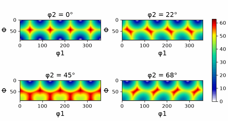
Each panel fixes the third Euler angle. The colour varies because the smallest angle to a cubic symmetry equivalent depends on all three Euler angles.
From a Harmonic Expansion
SO3FunHarmonic stores a finite harmonic series on \(SO(3)\). Converting the handle above at
bandwidth 16 retains harmonic degrees from 0 through 16.
SO3FHarmonic = SO3FunHarmonic(SO3FHandle, bandwidth=16)
SO3FHarmonic
SO3FunHarmonic (m3̅m → y↓→x)
  bandwidth: 16
  mean     : 40.7
plot(SO3FHarmonic, sections=4)
mtexColorbar()
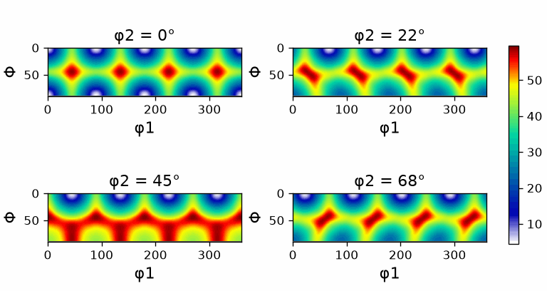
The broad pattern matches the handle plot. Sharp changes are rounded and may show oscillations because the series has been cut off at degree 16. Raising the bandwidth reduces this cut-off error at additional cost.
Currently, a bandwidth of up to 128 works reasonably fast in MTEX.
The power spectrum shows how much squared coefficient magnitude belongs to each harmonic degree.
plotSpectrum(SO3FHarmonic, lineWidth=2, figSize='small')
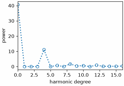
The plotted spectrum stops at degree 16 because higher coefficients were not retained. Its decay indicates how strongly the finer angular scales contribute to this approximation. See Harmonic Representation for coefficients and bandwidth in detail.
From Radial Functions
A radial function depends only on angular distance from a centre orientation. Examples include the de la Vallee Poussin, Abel–Poisson, Gauss–Weierstrass and von Mises–Fisher kernels.
Their common size parameter is the halfwidth. It is the angular distance at which the kernel value is half its value at the centre.
# define a de la Vallee Poussin kernel with 15 degree halfwidth
psi = SO3DeLaValleePoussinKernel(halfwidth=15 * degree)
psi
SO3DeLaValleePoussinKernel
  bandwidth: 17
  halfwidth: 15°
plot(psi)
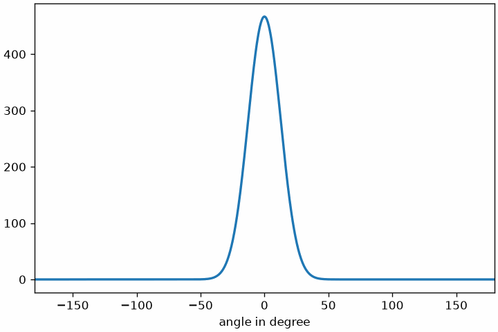
The curve is highest at zero angular distance and falls to half that height at 15 degrees. A smaller halfwidth therefore creates a narrower peak around every centre orientation.
A superposition of radial kernels can approximate a general function. Such SO3FunRBF
objects arise naturally in ODF reconstruction from pole figures and in kernel density
estimation from discrete orientations.
ori = orientation.rand(200, cs, rng=np.random.default_rng(1))

SO3FRBF = calcDensity(ori, kernel=psi)
SO3FRBF
SO3FunRBF (m3̅m → y↓→x)
  multimodal components
    kernel: de la Vallee Poussin, halfwidth 15°
    center: 200 orientations
    weight: 1
    Bunge Euler angles in degree
    phi1   Phi  phi2  weight
     274  82.9   251   0.005
    72.2   103   256   0.005
     142  54.3   143   0.005
    71.5  77.9  10.4   0.005
     202  43.7   166   0.005
       ⋮     ⋮     ⋮       ⋮
     251   114  31.3   0.005
     224  51.1   158   0.005
     262  93.8   349   0.005
     136   117  36.5   0.005
     170   115  48.3   0.005
plot(SO3FRBF, sections=4)
mtexColorbar()
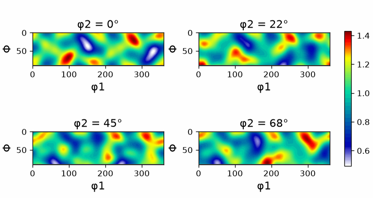
The density contains overlapping peaks centred at the 200 sampled orientations. Their 15
degree halfwidth smooths the individual samples into one continuous function. See
Radial ODFs for the weights, centres and kernels stored by SO3FunRBF.
From Fibre Components
A fibre is a one-dimensional family of orientations. SO3FunCBF represents a function as
a superposition of components distributed along such fibres, which is useful for modelling
a fibre ODF.
betaFibre = fibre.beta(cs)
betaFibre
fibre (m3̅m → y↓→x)
  h || r : [12 6 11] || (-1,-1,4)
  o1 → o2: (180°,35.26°,45°) → (270°,62.79°,45°)
SO3FCBF = SO3FunCBF(betaFibre, halfwidth=10 * degree)
SO3FCBF
SO3FunCBF (m3̅m → y↓→x)
  fibre component
    kernel: de la Vallee Poussin, halfwidth 10°
    fibre : (12 6 11) || (-0.231,-0.231,0.945), weight 1
    weight: 1
plot(SO3FCBF, sections=4)
mtexColorbar()
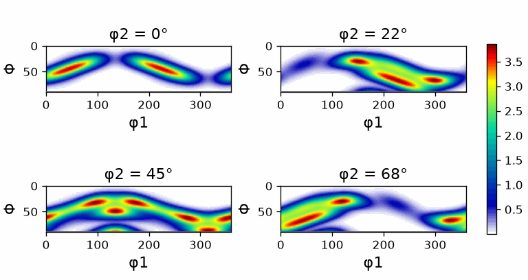
The high values follow the beta fibre through successive sections rather than forming an isolated orientation peak. The 10 degree halfwidth sets the spread transverse to that fibre. See Fibre ODFs for further constructions.
From a Bingham Distribution
A Bingham distribution is described by four
orientation axes U and four concentration values kappa. Together they specify the
directions and relative lengths of the half-axes of a four-dimensional ellipsoid.
kappa = [100, 90, 80, 0]
U = orientation.cat(orientation.byAxisAngle(xvector, np.array([0, 180]) * degree, cs),
                    orientation.byAxisAngle(vector3d.cat(yvector, zvector), 180 * degree, cs))
U
orientation (m3̅m → y↓→x)
  size: 4
  Bunge Euler angles in degree
  phi1  Phi  phi2
     0    0     0
     0  180     0
    90  180   270
   180    0     0
SO3FBingham = BinghamODF(kappa, U)
SO3FBingham
SO3FunBingham (m3̅m → y↓→x)
  kappa : [100.  90.  80.   0.]
  weight: 1
plot(SO3FBingham, sections=4)
mtexColorbar()
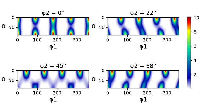
The unequal concentration values produce an anisotropic peak. Its shape differs along the four axes instead of depending only on distance from one centre. See Bingham ODFs for fitting and evaluation.
Vector-Valued Functions
The constructors above return scalar functions. Use SO3VectorField when every orientation should map to a vector instead of one number.
References
- H.-J. Bunge, Texture Analysis in Materials Science: Mathematical Methods, Butterworths, 1982, develops harmonic representations of orientation density functions.
- C. Bingham, An Antipodally Symmetric Distribution on the Sphere,
The Annals of Statistics 2 (1974), 1201-1225, introduces the distribution used by
SO3FunBingham.
Next
Continue with Operations on Orientation-Dependent Functions to evaluate, combine, differentiate and integrate the objects constructed here.
Technical Details
NumPy’s generator cannot reproduce MATLAB’s rng(1), so the 200 random orientations and
the density built from them differ from MATLAB’s.
Citing this page.
This page is part of the documentation of
MTEX, a free and open
source MATLAB toolbox for analyzing and modeling crystallographic textures.
It was written by The MTEX Developers and is published at
https://mtex-toolbox.github.io/SO3FunDefinition_py.html.
If you use MTEX, or reuse text or figures from this page, in your research,
please cite
F. Bachmann, R. Hielscher, H. Schaeben: Texture Analysis with MTEX - Free and Open Source Software Toolbox, Solid State Phenomena 160 (2010), 63-68. 10.4028/www.scientific.net/SSP.160.63
BibTeX
@article{bachmann2010mtex,
  author  = {F. Bachmann and R. Hielscher and H. Schaeben},
  title   = {Texture Analysis with MTEX - Free and Open Source Software Toolbox},
  journal = {Solid State Phenomena},
  volume  = {160},
  pages   = {63-68},
  year    = {2010},
  doi     = {10.4028/www.scientific.net/SSP.160.63},
  url     = {https://doi.org/10.4028/www.scientific.net/SSP.160.63}
}
Other papers describing specific MTEX methods are listed under Publications — please cite the one that best fits your application. The MTEX source code is licensed under the GNU General Public License v2.0; the text and figures of this documentation are licensed under CC BY 4.0, which permits reuse — including by automated systems — provided The MTEX Developers and this page are credited.