Radial ODFs

A radial orientation distribution function (ODF) is assembled from components whose value depends only on angular distance from a centre in orientation space. A uniform ODF is constant, a unimodal ODF has one centre, and a multimodal ODF is a sum of centred components.

MTEX stores all three as SO3FunRBF objects. Radial basis functions are a numerical representation, while uniform, unimodal, and multimodal describe the physical model. The objects still share the SO3Fun interface with every other ODF.

Here the centres are chosen deliberately. In Density Estimation, measured orientations become the centres of the same kind of sum. ODF Reconstruction may also return a radial-basis representation.

This page assumes the normalization introduced in ODF Theory and the model overview in ODF Modeling. The component shape is a kernel; Unimodal ODF Shapes compares the available choices.

from mtex import *

plottingConvention.default('y↑→x')

The Uniform ODF

The uniform ODF is the constant function

It represents an untextured specimen at 1 multiple of a random distribution (mrd) everywhere. Only the crystal and specimen symmetries are needed by uniformODF. The printed summary is useful here because it records both.

cs = crystalFrame('cubic')
ss = specimenFrame('orthorhombic')

odf = uniformODF(cs, ss)
odf

SO3FunRBF (m3̅m → y↑→x)
  uniform component
    weight: 1

One Radial Component

A unimodal ODF places one normalized peak at a preferred orientation. It needs the centre orientation, a kernel, and the crystal and specimen symmetries carried by that orientation. This example uses trivial specimen symmetry rather than assuming a sample symmetry that has not been shown.

cs = crystalFrame('432')
ss = specimenFrame()
mod1 = orientation.byMiller([1, 2, 2], [2, 2, 1], cs, ss)
psi = SO3vonMisesFisherKernel(halfwidth=10 * degree)

odf1 = unimodalODF(mod1, psi)
odf1

SO3FunRBF (432 → y↑→x)
  unimodal component
    kernel: von Mises Fisher, halfwidth 10°
    center: 1 orientation
    weight: 1
    Bunge Euler angles in degree
    phi1   Phi  phi2  weight
     297  48.2  26.6       1

The kernel halfwidth is the angular distance at which the peak has fallen to half its maximum. It is a spread parameter, not a cutoff. If the kernel is omitted, unimodalODF uses the de la Vallee Poussin kernel with a halfwidth of \(10^\circ\).

Several Radial Components

A second centre gives a second unimodal ODF with the same symmetry and kernel. Its terminated assignment suppresses a summary identical in form to the one above.

mod2 = orientation.byMiller([1, 1, 2], [0, 2, 1], cs, ss)
odf2 = unimodalODF(mod2, psi)

Adding the two functions gives a multimodal ODF. The summary shows that MTEX keeps the result as one radial-basis object with several centres.

odf3 = odf1 + odf2
odf3

SO3FunRBF (432 → y↑→x)
  multimodal components
    kernel: von Mises Fisher, halfwidth 10°
    center: 2 orientations
    weight: 2
    Bunge Euler angles in degree
    phi1   Phi  phi2  weight
     297  48.2  26.6       1
     231  35.3    45       1

Each input has mean 1, so an unscaled sum has mean 2 rather than 1. It is therefore not a normalized ODF.

mean(odf3)

2

Compare the two components and their sum on one shared colour range. The top row contains the {100} pole figures and the bottom row the {110} pole figures. The columns show the first component, second component, and sum.

h = cat(Miller(1, 0, 0, cs), Miller(1, 1, 0, cs))
odfParts = [odf1, odf2, odf3]
partName = ['first component', 'second component', 'sum']

mtexFig = newMtexFigure(layout=[2, 3])
for i in range(h.size):
  for j in range(len(odfParts)):
    plotPF(odfParts[j], h[i], antipodal=True, title=False)
    mtexTitle(partName[j])
    if i < h.size - 1 or j < len(odfParts) - 1:
      nextAxis()
setColorRange('equal')
mtexColorbar(title='mrd')

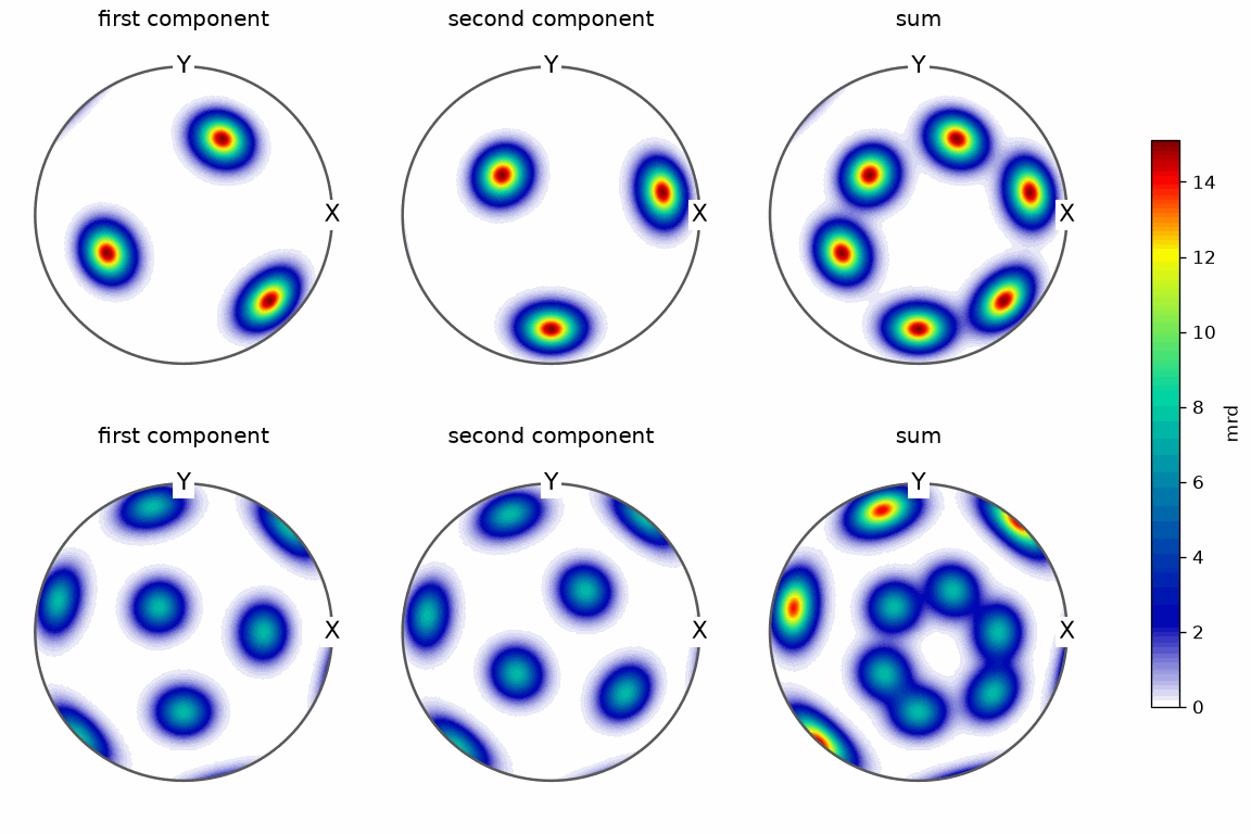
Each centre produces one set of symmetry-equivalent spots per pole figure. Those copies are one physical component, not additional modes. In the sum, both sets remain because each component entered with coefficient 1. Where spots overlap, the summed patch becomes stronger or elongated; that overlap is not a third centre.

Mixture Weights

A normalized mixture scales individually normalized components by coefficients that sum to one. These coefficients are component volume fractions, even when the peaks overlap in orientation space. Equal shares would be 0.5*odf1 + 0.5*odf2; the unequal mixture below shows that each component may have a weight of its own.

odf4 = 0.25 * odf1 + 0.75 * odf2
odf4

SO3FunRBF (432 → y↑→x)
  multimodal components
    kernel: von Mises Fisher, halfwidth 10°
    center: 2 orientations
    weight: 1
    Bunge Euler angles in degree
    phi1   Phi  phi2  weight
     297  48.2  26.6    0.25
     231  35.3    45    0.75

The mean is 1 again. Any number of centred components can be combined in the same way, with a coefficient of its own. Once a model is built, ODF Properties extracts its modes, volume fractions, and texture strength.

mean(odf4)

1

The Maths Behind Radial Components

For a centre \(x\), a radial component has the form

where \(\omega(g,x)\) is the symmetry-aware angular distance between the orientations. Crystal and specimen symmetry therefore repeat the same physical centre at its equivalent descriptions automatically.

More generally, a radial-basis ODF is stored as

The constant \(c_0\) gives the uniform part. One nonzero weight gives a unimodal ODF, and several weights give a multimodal ODF. This is why adding radial ODFs does not require changing representation.

Further Reading

• Hielscher (2013) develops kernel density estimation on the rotation group and compares kernel families for crystallographic texture analysis.
• Hielscher and Schaeben (2008) explains the radially symmetric discretization used in the MTEX pole figure inversion algorithm.

Next

The kernels that give these peaks their shape are Unimodal ODF Shapes. A peak spread along a curve rather than about a point is a Fibre ODF.

Technical Details

The display of a radial function names its kernel, the number of centres and their total weight where MATLAB prints the table of Euler angles. MATLAB’s drawNow has no counterpart, the figure is drawn when it is shown.

@article{bachmann2010mtex,
  author  = {F. Bachmann and R. Hielscher and H. Schaeben},
  title   = {Texture Analysis with MTEX - Free and Open Source Software Toolbox},
  journal = {Solid State Phenomena},
  volume  = {160},
  pages   = {63-68},
  year    = {2010},
  doi     = {10.4028/www.scientific.net/SSP.160.63},
  url     = {https://doi.org/10.4028/www.scientific.net/SSP.160.63}
}