
An orientation distribution function (ODF) does not have to come from a measurement. A model ODF is built from a few chosen ingredients: a preferred orientation and its spread, a fibre, or a mixture of these. Because its ingredients are known, a model ODF can serve as a reference for measured textures, as a starting point for texture-evolution simulations, or as test data with a known answer.
This page assumes the normalization and multiples of a random distribution (mrd) introduced in ODF Theory. Every ODF in MTEX follows the SO3Fun interface for functions on the rotation group \(SO(3)\). The physical model and its numerical representation are related, but they are not the same choice:
| construction | meaning |
|---|---|
| uniform | constant, the untextured reference |
| unimodal | a radial peak about one orientation |
| multimodal | several radial peaks |
| fibre | a peak spread along a curve in orientation space |
| Bingham | a parametric peak with three independent spreads |
| harmonic representation | a series expansion, the classical form used for pole figure inversion |
Harmonic names a representation, not another physical peak shape. The current calcODF normally returns a radial-basis ODF. It can then be converted to a harmonic series. All of these objects share one interface for evaluation, plotting, scaling, and addition. This is why components with different representations can be mixed in one model.
from mtex import *
plottingConvention.default('y↑→x')
The Uniform ODF
The simplest model is the constant function
\[f(g) = 1,\quad g \in SO(3).\]It needs only the crystal and specimen symmetries. The returned summary is useful here: it records both symmetries and identifies the constant component.
cs = crystalFrame('cubic')
ss = specimenFrame('orthorhombic')

odf = uniformODF(cs, ss)
odf
SO3FunRBF (m3̅m → y↑→x)
  uniform component
    weight: 1
A value of 1 mrd everywhere is an untextured specimen. This uniform ODF is the reference against which every other mrd value is measured.
A Single Component
A unimodal ODF is a peak about one preferred orientation. A kernel sets the shape, and its halfwidth sets the angular distance at which the kernel falls to half its maximum. The halfwidth is a spread parameter, not a cutoff: the component continues beyond that angle.
psi = SO3vonMisesFisherKernel(halfwidth=10 * degree)

mod1 = orientation.byMiller([1, 2, 2], [2, 2, 1], cs, ss)

odf1 = unimodalODF(mod1, psi)
odf1
SO3FunRBF (m3̅m → y↑→x)
  unimodal component
    kernel: von Mises Fisher, halfwidth 10°
    center: 1 orientation
    weight: 1
    Bunge Euler angles in degree
    phi1   Phi  phi2  weight
     297  48.2  26.6       1
The summary records the kernel, centre, and component weight. The maximum sits at the preferred orientation and its symmetry-equivalent copies. Its value measures concentration rather than volume fraction. A narrower normalized peak has a higher maximum because its mean must remain one.
odfMax = max(odf1)[0]
odfMax
15.9612
plotPF(odf1, cat(Miller(1, 0, 0, cs), Miller(1, 1, 0, cs)), antipodal=True, colorRange='equal')
mtexColorbar(title='mrd')
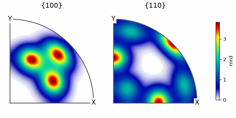
The localized spots are projections of one preferred orientation and its symmetry-equivalent copies. They are not separate components.
Mixtures
ODFs are added and scaled like functions, so a textured component can sit on a uniform background. The classical Santa Fe standard is 27 percent of the component above and 73 percent uniform background.
odf = 0.73 * uniformODF(cs, ss) + 0.27 * unimodalODF(mod1, psi)
odf
SO3FunRBF (m3̅m → y↑→x)
  uniform component
    weight: 0.73
  unimodal component
    kernel: von Mises Fisher, halfwidth 10°
    center: 1 orientation
    weight: 0.27
    Bunge Euler angles in degree
    phi1   Phi  phi2  weight
     297  48.2  26.6    0.27
The printed summary separates the uniform and unimodal terms. Both are individually normalized, so their coefficients act as mixture volume fractions. They must add up to one if the mixture is to remain normalized.
mean(odf)
1
The mean is 1. The component peaks may overlap in orientation space, but the coefficients still describe the fractions assigned to the two terms. They are not volumes of disjoint regions drawn around the maxima.
plotPF(odf, cat(Miller(1, 0, 0, cs), Miller(1, 1, 0, cs)), antipodal=True, colorRange='equal')
mtexColorbar(title='mrd')
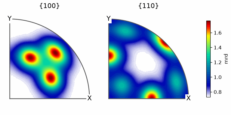
The uniform term contributes a 0.73 mrd background, while the unimodal term produces the spots. This known model is commonly used to test pole figure inversion; The Santa Fe Example simulates pole figures from it and scores the reconstruction against the answer.
Rotating a Model
rotate actively moves a model relative to the specimen axes. By default, the rotation acts on the specimen side of every component orientation.
odfRot = rotate(odf, rotation.byAxisAngle(vector3d.Z, 30 * degree))

plotPF(odfRot, cat(Miller(1, 0, 0, cs), Miller(1, 1, 0, cs)), antipodal=True, colorRange='equal')
mtexColorbar(title='mrd')
Warning: Rotating an ODF with specimen symmetry will remove the specimen symmetry
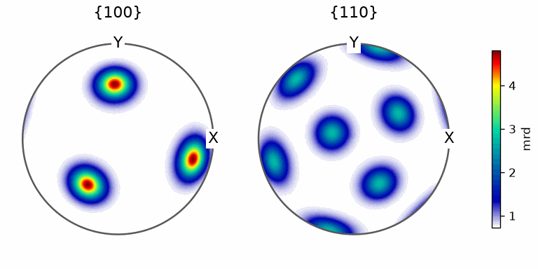
Compared with the preceding pole figures, every feature turns by \(30^\circ\) about the
centre. The original mmm specimen symmetry was tied to x, y, and z. It is no longer
coordinate-aligned after this rotation, so MTEX drops the specimen-symmetry label and
issues a warning. The physical twofold axes have rotated with the texture.
A frame change is different: it re-expresses the same physical texture in another reference frame and leaves the texture itself untouched. Use transformReferenceFrame when the crystal frame changes. The corresponding coordinate transformation is inverse to an active rotation.
Further Reading
- Bunge, Texture Analysis in Materials Science develops the mathematical foundations of ODFs and their representations.
- Matthies, Vinel, and Helming, Standard Distributions in Texture Analysis is an atlas of cubic-orthorhombic model textures.
- Roe (1965) gives the classical harmonic solution of the pole figure inversion problem.
- Kunze and Schaeben (2004) develop quaternion Bingham distributions for texture analysis.
Next
Plotting an ODF compares the views used to inspect these models. The model-family pages begin with Radial ODFs. Fibre ODFs and Bingham ODFs cover the other shapes listed above. Random Sampling turns a model back into discrete orientations, while Properties extracts the numbers that describe any ODF.
Technical Details
The sum of a uniform and a unimodal radial function stays one SO3FunRBF, as in MATLAB;
the port lists the uniform part and the kernel centres in its display without MATLAB’s
table of Euler angles. max(odf) returns the pair of the value and the orientation.
Citing this page.
This page is part of the documentation of
MTEX, a free and open
source MATLAB toolbox for analyzing and modeling crystallographic textures.
It was written by The MTEX Developers and is published at
https://mtex-toolbox.github.io/ODFModeling_py.html.
If you use MTEX, or reuse text or figures from this page, in your research,
please cite
F. Bachmann, R. Hielscher, H. Schaeben: Texture Analysis with MTEX - Free and Open Source Software Toolbox, Solid State Phenomena 160 (2010), 63-68. 10.4028/www.scientific.net/SSP.160.63
BibTeX
@article{bachmann2010mtex,
  author  = {F. Bachmann and R. Hielscher and H. Schaeben},
  title   = {Texture Analysis with MTEX - Free and Open Source Software Toolbox},
  journal = {Solid State Phenomena},
  volume  = {160},
  pages   = {63-68},
  year    = {2010},
  doi     = {10.4028/www.scientific.net/SSP.160.63},
  url     = {https://doi.org/10.4028/www.scientific.net/SSP.160.63}
}
Other papers describing specific MTEX methods are listed under Publications — please cite the one that best fits your application. The MTEX source code is licensed under the GNU General Public License v2.0; the text and figures of this documentation are licensed under CC BY 4.0, which permits reuse — including by automated systems — provided The MTEX Developers and this page are credited.