
An orientation-dependent function assigns a numerical value to every rotation or crystal
orientation. The set of rotations is the rotation group \(SO(3)\), which gives the MTEX class
SO3Fun its name.
An important example is the orientation density function (ODF). It assigns a density to each crystal orientation in a specimen. Other examples include the Schmid factor and the Taylor factor as functions of crystal orientation.
A First Orientation-Dependent Function
MTEX represents a scalar function on \(SO(3)\) by an object of type SO3Fun. Its symmetries determine which rotations represent the same argument.
Consider the smallest rotational angle between an orientation and the identity, including
its cubic symmetry equivalents. The angle command returns this
angle in radians. Dividing by degree makes the function value a number in degrees.
import numpy as np

from mtex import *

# define cubic crystal symmetry
cs = crystalFrame('432')

# wrap the angle formula in an SO3Fun
SO3F = SO3FunHandle(lambda ori: angle(ori) / degree, cs)
SO3F
SO3FunHandle (432 → y↓→x)
  bandwidth hint: 64
Evaluate the Function
SO3FunHandle turns a Python function into an SO3Fun. The variable SO3F now stores
the formula together with its symmetry.
Use eval to evaluate it at one or many orientations. Here the input is fixed so that the result is reproducible.
ori = orientation.byEuler(20 * degree, 30 * degree, 10 * degree, cs)
ori
orientation (432 → y↓→x)
  Bunge Euler angles in degree
  phi1  Phi  phi2
    20   30    10
angleInDegrees = SO3F.eval(ori)
angleInDegrees
42.1812
The returned scalar is the smallest angle, in degrees, among the symmetrically equivalent
representatives of ori. The next page develops this construction and the other ways to
define an SO3Fun.
Plot Euler-Angle Sections
A scalar function on \(SO(3)\) depends on three coordinates. MTEX can show it as a stack of sections at fixed third Euler angle \(\varphi_2\).
plotSection(SO3F, sections=4)
mtexColorbar()
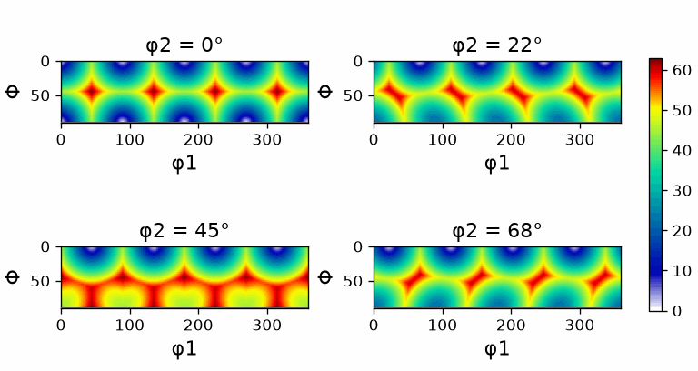
Each panel covers the first two Euler angles at one value of \(\varphi_2\). The colour changes within and between panels because the smallest symmetry-reduced angle depends on all three Euler angles.
Plot Axis–Angle Sections
The same function is especially simple in axis–angle coordinates. Each section fixes the rotational angle and varies the rotational axis.
plotSection(SO3F, 'axisAngle', np.arange(15, 61, 15) * degree, pcolor=True)
mtexColorbar()
mtexColorMap('parula')
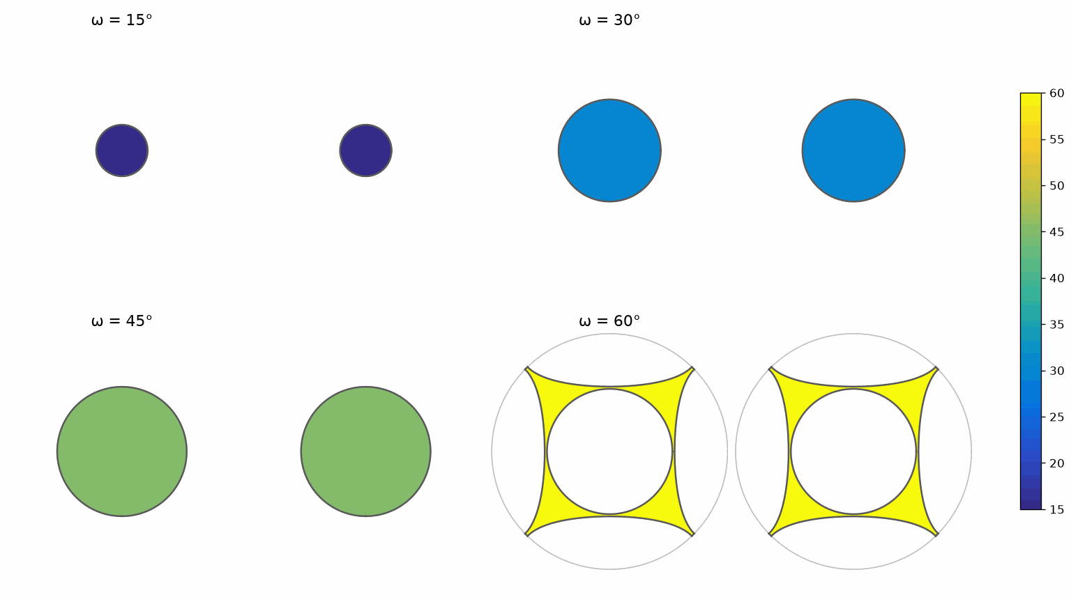
Every panel has one colour because SO3F returns the angle that labels that panel. A
rotation by one of these angles may have any axis, so each angle fills the whole sphere
and needs an upper and a lower panel. The two section plots show the same function in
different coordinates; neither changes the underlying data.
Analyse an Orientation-Dependent Function
The common SO3Fun interface provides arithmetic, integration, differentiation and
searches for extrema. For this angle function, a local maximum is an orientation farthest
from a cubic symmetry equivalent of the identity.
The max command below requests up to ten distinct local maxima. The
accuracy option controls the final angular search tolerance.
value, oriMax = max(SO3F, numLocal=10, accuracy=0.001 * degree)
value
array([62.7994, 62.7994, 62.7994, 62.7993, 62.7993, 62.7993])
oriMax
orientation (432 → y↓→x)
  size: 6
  Bunge Euler angles in degree
  phi1  Phi  phi2
   270   45    45
    45   45   270
   135   45   180
   215   60   125
   180   45   135
   360   45   315
The calculation finds exactly six symmetrically inequivalent maxima. Their function values are about 62.799 degrees, and their positions are the vertices of the fundamental region in orientation space.
color = ind2color(np.tile(np.arange(oriMax.size), (numSym(cs), 1)))
plot(oriMax.symmetrise(), color, 'axisAngle', filled=True, markerSize=20, fundamentalRegion=True)
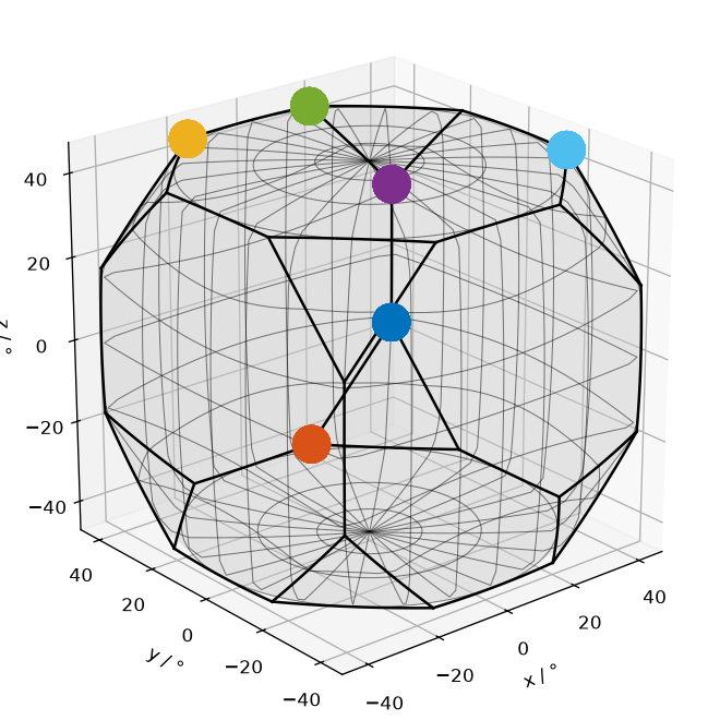
The six colours distinguish the six maxima. The markers lie on the outer vertices because those points have the greatest possible distance from the identity after cubic symmetry has been taken into account.
Representations of Orientation-Dependent Functions
MTEX can store a function in several ways. The representation controls how the function
is constructed and how expensive an operation is, but all representations share the
SO3Fun interface.
| representation | MTEX class or documentation |
|---|---|
| harmonic series expansion | SO3FunHarmonic |
| superposition of radial functions | SO3FunRBF |
| superposition of fibre elements | SO3FunCBF |
| Bingham distribution | SO3FunBingham |
| sum of different components | SO3FunComposition |
| formula evaluated on demand | SO3FunHandle |
Thus functions with different internal representations can be added, multiplied, averaged, integrated or differentiated through the same API.
Related Function Types
SO3VectorField assigns a vector instead of a scalar to each rotation. SO3Kernel represents a radial function whose value depends only on rotational angle.
References
- H.-J. Bunge, Texture Analysis in Materials Science: Mathematical Methods, Butterworths, 1982, develops the orientation-space and ODF framework used here.
Next
Continue with Defining Orientation-Dependent Functions to construct functions from formulas, harmonic coefficients and sampled values.
Technical Details
The maxima lie within \(10^{-4}\) degree of the vertices of the fundamental region, where the region’s faces meet; the symmetric copies of one maximum are therefore folded onto different equivalent vertices of the region’s surface, which the plot shows in the colour of that maximum, where MATLAB’s run shows one marker per maximum. MATLAB lists the maxima in other symmetric equivalents.
Citing this page.
This page is part of the documentation of
MTEX, a free and open
source MATLAB toolbox for analyzing and modeling crystallographic textures.
It was written by The MTEX Developers and is published at
https://mtex-toolbox.github.io/SO3FunConcept_py.html.
If you use MTEX, or reuse text or figures from this page, in your research,
please cite
F. Bachmann, R. Hielscher, H. Schaeben: Texture Analysis with MTEX - Free and Open Source Software Toolbox, Solid State Phenomena 160 (2010), 63-68. 10.4028/www.scientific.net/SSP.160.63
BibTeX
@article{bachmann2010mtex,
  author  = {F. Bachmann and R. Hielscher and H. Schaeben},
  title   = {Texture Analysis with MTEX - Free and Open Source Software Toolbox},
  journal = {Solid State Phenomena},
  volume  = {160},
  pages   = {63-68},
  year    = {2010},
  doi     = {10.4028/www.scientific.net/SSP.160.63},
  url     = {https://doi.org/10.4028/www.scientific.net/SSP.160.63}
}
Other papers describing specific MTEX methods are listed under Publications — please cite the one that best fits your application. The MTEX source code is licensed under the GNU General Public License v2.0; the text and figures of this documentation are licensed under CC BY 4.0, which permits reuse — including by automated systems — provided The MTEX Developers and this page are credited.