
A vector field on the rotation group assigns a tangent vector to every orientation.
Evaluating an SO3VectorField at an orientation \(R\) returns an SO3TangentVector
attached to \(R\).
Read The Tangent Space on the Rotation Group first for the definition of tangent vectors and their left and right representations. Vector fields model orientation-dependent spin in Taylor and Sachs calculations. The gradient of an orientation distribution function (ODF) is another important example.
import numpy as np

from mtex import *

plottingConvention.default('y↑→x')
A first vector field: the gradient of an ODF
Consider the model ODF for a quartz specimen known as the Dubna texture. The gradient points in the direction of the fastest local increase of the ODF, and its norm gives that rate of increase.
odf = SO3Fun.dubna()
G = odf.grad()
G
SO3VectorFieldHarmonic (Quartz → y↑→x)
  tangent space: left
  bandwidth    : 48
Evaluation at one sampled orientation returns the tangent vector attached to that orientation.
rng = np.random.default_rng(1)
ori = odf.discreteSample(1, rng=rng)
G.eval(ori)
SO3TangentVector (left, y↑→x)
  reference: orientation (Quartz → y↑→x), one per element
    x    y     z
  -66  117  86.1
Plot the ODF in sigma sections and draw the gradient arrows on top.
plot(odf, 'sigma')
hold('on')
plot(G, lineWidth=1.5, color='black', resolution=7.5 * degree)
hold('off')
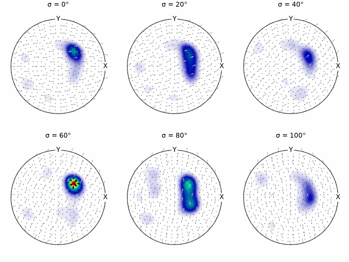
The arrows point uphill towards the nearest local maximum. Their lengths increase where the ODF changes more steeply. This ascent direction is the basis of the steepest-descent algorithm used by max and calcComponents.
Three representations
MTEX provides three interchangeable representations. A harmonic or RBF field stores three scalar component functions using the array convention introduced in Vector-Valued Orientation Functions.
| representation | class | when to use it |
|---|---|---|
| three harmonic component functions | SO3VectorFieldHarmonic | differentiation and global spectral approximation |
| three radial-basis component functions | SO3VectorFieldRBF | approximation by local kernels |
| an evaluation formula | SO3VectorFieldHandle | an explicit rule that can be evaluated at any orientation |
All three representations support the common SO3VectorField operations.
Left and right tangent-vector coordinates
An SO3VectorField has a requested tangent-space representation and two associated
symmetries. Left coordinates are the default. The right and
left methods re-express the same geometric vectors; they do
not change the vectors or their base orientations.
GR = right(G)
GR
SO3VectorFieldHarmonic (Quartz → y↑→x)
  tangent space: right
  bandwidth    : 49
v = GR.eval(ori)
vRight = right(G.eval(ori))
norm(v - vRight)
array([0.])
The small residual shows that converting the field before evaluation and converting the evaluated tangent vector give the same result. Arithmetic also converts compatible fields to a common representation automatically.
G + GR
SO3VectorFieldHarmonic (Quartz → y↑→x)
  tangent space: left
  bandwidth    : 49
Why the visible symmetries change
A field’s tangent vectors live in the frame of one side: left vectors in the specimen frame, right vectors in the crystal frame. Symmetry acts differently on the two coordinate choices. For a right-represented tangent vector, evaluations at symmetry-equivalent orientations are meaningful only with respect to the left symmetry. For a left-represented tangent vector, the reverse applies.
ori = orientation.rand(G.CS, G.SS, rng=rng)
G.eval(ori.symmetrise())
SO3TangentVector (left, y↑→x)
  size     : 6
  reference: orientation (Quartz → y↑→x), one per element
        x     y        z
  0.00289  0.05  -0.0189
  0.00289  0.05  -0.0189
  0.00289  0.05  -0.0189
  0.00289  0.05  -0.0189
  0.00289  0.05  -0.0189
  0.00289  0.05  -0.0189
GR.eval(ori.symmetrise())
SO3TangentVector (right, Quartz)
  size     : 6
  reference: orientation (Quartz → y↑→x), one per element
        x        y        z
   0.0134  -0.0467   0.0226
  -0.0471   0.0117   0.0226
   0.0471   0.0117  -0.0226
   0.0337    0.035   0.0226
  -0.0337    0.035  -0.0226
  -0.0134  -0.0467  -0.0226
The left vectors turn with the crystal symmetry operation that relates the equivalent orientations, while the right vectors, given in crystal coordinates, repeat. The field keeps the crystal and specimen frames of the ODF either way, and the component functions of each side carry the symmetry that side leaves them.
Operations on vector fields
The following operations apply to vector fields VF, VF1 and VF2:
- sums, differences, scaling and division
- inner products with dot(VF1, VF2)
- cross products with cross(VF1, VF2)
- norms with norm(VF)
- normalization with normalize(VF)
- rotation with rotate(VF, rot)
- averages with mean(VF)
Since a gradient is itself a vector field, MTEX can also compute its divergence, curl and scalar antiderivative.
Divergence and the Laplacian
Treating G as an orientation-space velocity field gives an intuitive reading of its
divergence. Negative divergence marks a sink where nearby orientations condense. Positive
divergence marks a source where they spread apart.
The divergence of a gradient equals the Laplacian of its scalar field. Plot the two calculations side by side at the same sigma section.
plot(G.div(), 'sigma', 60 * degree)
nextAxis()
plot(laplace(SO3FunHarmonic(odf)), 'sigma', 60 * degree)
mtexColorbar()
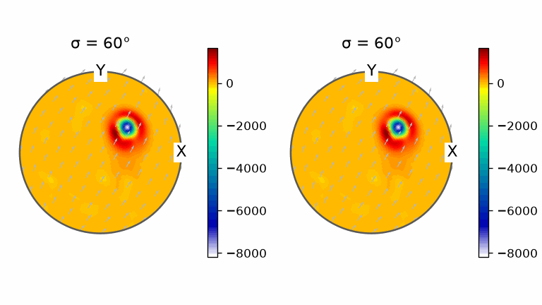
The source and sink regions, contour shapes and colour scale agree in the two panels. The left panel was computed from the vector field, whereas the right panel was computed directly from the ODF.
Curl and conservative fields
Curl describes the axis of local circulation within orientation space. The curl of a gradient is zero, so the next plot should contain no nonzero arrows.
plot(G.curl(), 'sigma')
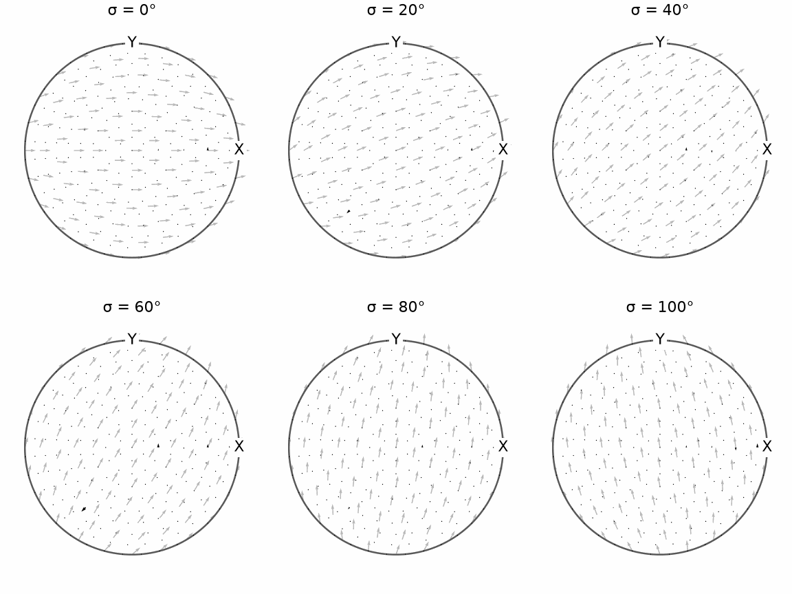
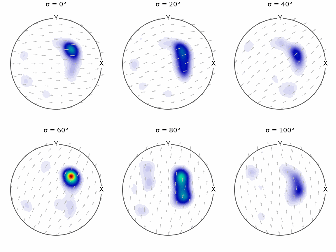
Vanishing curl identifies a conservative field: a field that is the gradient of a scalar potential. The antiderivative method reconstructs that potential.
odf2 = G.antiderivative()
odf2
SO3FunHarmonic (Quartz → y↑→x)
  bandwidth: 48
  mean     : 0
A gradient loses the additive constant of its source function. Restoring the original
mean makes the reconstructed potential coincide with odf.
odf2 = odf2 + mean(odf)
plot(odf2, 'sigma')
Define a field by an evaluation formula
A Python function is convenient when a vector formula is known. The following rule uses the rotation axis multiplied by the rotation angle, with cubic symmetry on both sides.
cs = crystalFrame('432')
cs
crystalFrame (⊙c→a)
  symmetry: 432
  elements: 24
  a, b, c : 1, 1, 1
f = lambda mori: mori.axis() * mori.angle()
VF = SO3VectorFieldHandle(f, cs, cs)
VF
SO3VectorFieldHandle (432 → 432)
  tangent space : left
  bandwidth hint: 64
Evaluating a \(10^\circ\) rotation about \([1\;2\;3]\) and reducing the axis to small integers recovers the expected direction ratio \(1:2:3\).
round(VF.eval(orientation.byAxisAngle(vector3d(1, 2, 3), 10 * degree, cs, cs)))
SO3TangentVector (left, 432)
  reference: misorientation (432 → 432)
  x  y  z
  1  2  3
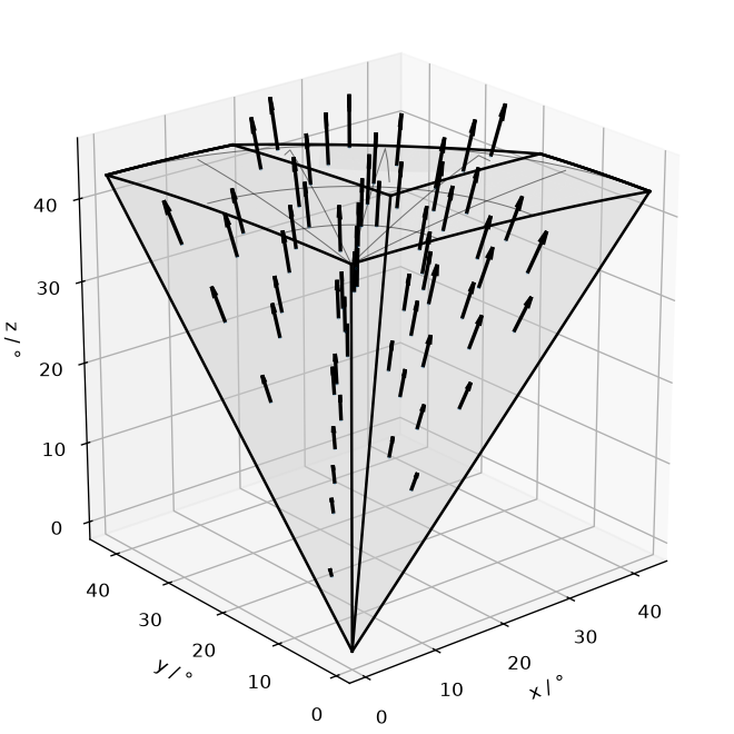
The following axis-angle plot samples the formula throughout the cubic fundamental region. Every arrow points away from the identity at the origin, as a field of axis times angle must.
quiver3d(VF, 'axisAngle', resolution=7.5 * degree, color='black', lineWidth=2)
Convert a field to harmonic form
Passing any SO3VectorField to the harmonic constructor expands its three components by
quadrature.
SO3VectorFieldHarmonic(VF)
SO3VectorFieldHarmonic (432 → 432)
  tangent space: left
  bandwidth    : 64
Fit harmonic components to sampled values
A second construction starts from rotations and one vector3d value at each rotation. The
first array dimension again corresponds to nodes.
nodes = equispacedSO3Grid(specimenFrame('1'), points=1e3).flatten()
y = vector3d.byPolar(np.sin(3 * nodes.angle()), nodes.phi2 + np.pi / 2)
The approximation below produces a harmonic vector field with bandwidth 16.
SO3VF1 = SO3VectorFieldHarmonic.approximate(nodes, y, bandwidth=16)
SO3VF1
SO3VectorFieldHarmonic (y↑→x → y↑→x)
  tangent space: left
  bandwidth    : 16
Construct by quadrature of a function
A function that accepts a rotation and returns a vector3d can also be passed directly to
quadrature. Here the earlier cubic formula produces a harmonic vector field.
SO3VF2 = SO3VectorFieldHarmonic.quadrature(lambda v: f(v))
SO3VF2
SO3VectorFieldHarmonic (1 → y↑→x)
  tangent space: left
  bandwidth    : 64
Construct from three scalar harmonic functions
A three-component SO3FunHarmonic can be wrapped directly. Its first, second and third
entries become the \(x\), \(y\) and \(z\) components of the vector field.
SO3F = SO3FunHarmonic(rng.random((3, 1000)))
SO3F
SO3FunHarmonic (1 → y↑→x)
  size     : 3
  bandwidth: 9
  isReal   : false
SO3VF3 = SO3VectorFieldHarmonic(SO3F)
SO3VF3
SO3VectorFieldHarmonic (1 → y↑→x)
  tangent space: left
  bandwidth    : 9
Application: orientation-dependent spin in the Taylor model
Taylor theory accommodates a prescribed strain by activating slip systems in each crystal.
The antisymmetric part of the resulting deformation describes the local lattice spin, and
therefore the local misorientation predicted for each orientation. Without an input
orientation, calcTaylor returns this spin as an
SO3VectorField.
cs = crystalFrame('432')
sS = slipSystem.bcc(cs)
sS
slipSystem (432)
  size: 3
   u   v  w  | h  k  l  CRSS
   1  -1  1    0  1  1     1
  -1   1  1    2  1  1     1
  -1   1  1    3  2  1     1
Set plane strain with \(q=0\) and calculate the spin field for the symmetrised body-centred-cubic slip systems.
q = 0
epsilon = strainTensor(np.diag([1, -q, -(1 - q)]))
epsilon
strainTensor (y↑→x)
  rank: 2 (3 × 3)
  1  0   0
  0  0   0
  0  0  -1
_, _, W = calcTaylor(epsilon, sS.symmetrise())
W
SO3VectorFieldHarmonic (432 → y↑→x)
  tangent space: left
  bandwidth    : 32
Display the spin directions in four Euler-angle sections.
sP = phi1Sections(cs, specimenFrame('222'))
sP.phi1 = np.arange(10, 71, 20) * degree
plot(W, sP, resolution=7.5 * degree, layout=[2, 2])
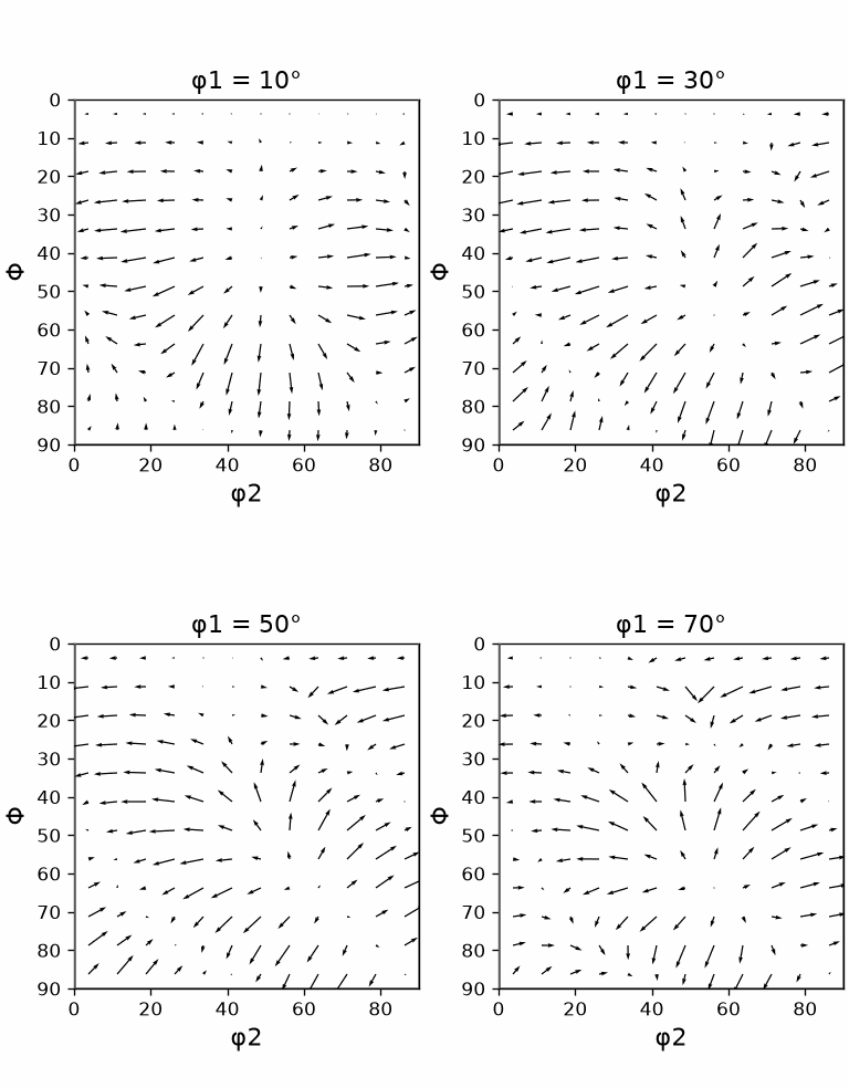
Direction and length vary with orientation, showing that the Taylor model predicts a different local misorientation across orientation space. The value at the copper orientation can be retrieved directly.
WCopper = W.eval(orientation.copper(cs))
WCopper
SO3TangentVector (left, y↑→x)
  reference: orientation (432 → y↑→x)
          x       y         z
  -2.97e-10  -0.464  1.34e-09
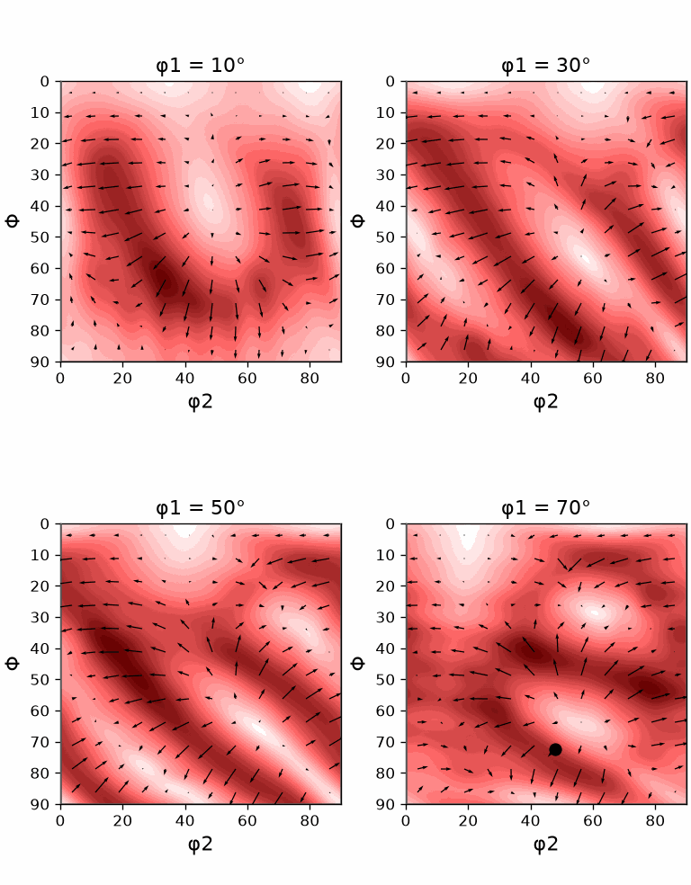
The amount of spin
The norm of the spin vector is the angle of local misorientation. Its maximum locates the orientation with the largest predicted rotation.
_, oriMax = max(norm(W))
oriMax
orientation (432 → y↑→x)
  Bunge Euler angles in degree
  phi1   Phi  phi2
  55.8  50.3   293
Plot the norm at \(0.5^\circ\) resolution and overlay the more coarsely sampled vector
field. The background shows magnitude, the arrows show direction, and the annotation marks
oriMax.
plot(norm(W), sP, resolution=0.5 * degree, layout=[2, 2])
mtexColorMap('LaboTeX')
hold('on')
plot(W, sP, resolution=7.5 * degree, color='black')
hold('off')
annotate(oriMax)
Compare spin with a crystal direction
Since W gives the rotation axis of the local misorientation, its inner product with a
chosen direction measures signed alignment. Here the direction is crystal \([100]\).
plot(dot(W, Miller(1, 0, 0, cs)), sP, layout=[2, 2])
mtexColorMap('blue2red')
mtexColorbar()
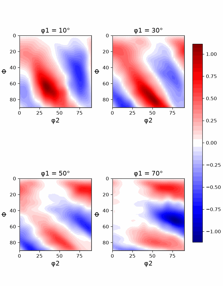
Positive and negative regions indicate parallel and antiparallel components along \([100]\). Values near zero indicate that the spin axis is locally perpendicular to that direction.
Sources and sinks of the Taylor spin field
Finally compute the divergence of W. As in the gradient example, negative values are
sinks and positive values are sources in orientation space.
flux = W.div()
flux
SO3FunHarmonic (432 → y↑→x)
  bandwidth: 32
  mean     : 0
plot(flux, sP, resolution=0.5 * degree, layout=[2, 2], faceAlpha=0.5)
mtexColorMap('blue2red')
mtexColorbar()
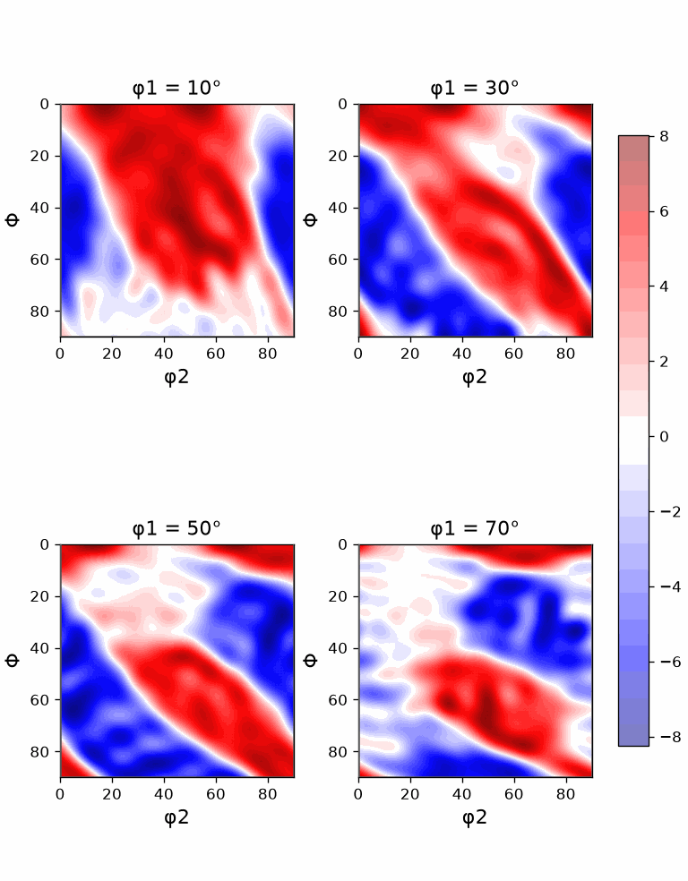
The alternating red and blue regions show that the Taylor spin field moves orientations towards some parts of orientation space and away from others.
References
- A. Morawiec, Orientations and Rotations: Computations in Crystallographic Textures, Springer, 2004, develops the tangent-space geometry used for gradients and vector fields on \(\mathrm{SO}(3)\).
- H.-J. Bunge, Some applications of the Taylor theory of polycrystal plasticity, Kristall und Technik 5 (1970), 145–175, gives the orientation-dependent Taylor factors and spin fields used in the final example.
Next
Continue with Rotational Kernel Functions to understand the localized basis functions used by the RBF representation listed on this page.
Technical Details
A field in the port keeps its crystal and specimen frames on either side; MATLAB’s hidden
symmetries are the groups the component functions carry. A field is stored on the side it
is given in, so right(G) is a field of its own at bandwidth 49 where MATLAB keeps the
left one at 48 and converts on evaluation. The Taylor spin field is in left components, as
the Julia port keeps it, where MATLAB shows the right spin tensor: the copper spin
\((0, -0.463, 0)\) in specimen coordinates stands for MATLAB’s tensor with entries
\(\pm 0.3215\) in crystal coordinates, a vector of length 0.455. dot(W, Miller(1, 0, 0, cs))
of the left field takes its right components, since a crystal direction lives in the
crystal frame. The largest spin is found at \((259^\circ, 42.4^\circ, 123^\circ)\) with 1.207,
MATLAB’s at \((268.7^\circ, 45.4^\circ, 63.3^\circ)\), where the port’s field has 1.173, 9.4
degrees away under the symmetry of the strain. MATLAB’s cached Dubna ODF keeps the
plotting convention y↓→x of an earlier session, the port’s follows the page’s y↑→x, so
the sigma sections of the gradient are MATLAB’s turned by 180 degrees about z. The sampled
orientation and the random coefficients come from NumPy.
Citing this page.
This page is part of the documentation of
MTEX, a free and open
source MATLAB toolbox for analyzing and modeling crystallographic textures.
It was written by The MTEX Developers and is published at
https://mtex-toolbox.github.io/SO3FunVectorField_py.html.
If you use MTEX, or reuse text or figures from this page, in your research,
please cite
F. Bachmann, R. Hielscher, H. Schaeben: Texture Analysis with MTEX - Free and Open Source Software Toolbox, Solid State Phenomena 160 (2010), 63-68. 10.4028/www.scientific.net/SSP.160.63
BibTeX
@article{bachmann2010mtex,
  author  = {F. Bachmann and R. Hielscher and H. Schaeben},
  title   = {Texture Analysis with MTEX - Free and Open Source Software Toolbox},
  journal = {Solid State Phenomena},
  volume  = {160},
  pages   = {63-68},
  year    = {2010},
  doi     = {10.4028/www.scientific.net/SSP.160.63},
  url     = {https://doi.org/10.4028/www.scientific.net/SSP.160.63}
}
Other papers describing specific MTEX methods are listed under Publications — please cite the one that best fits your application. The MTEX source code is licensed under the GNU General Public License v2.0; the text and figures of this documentation are licensed under CC BY 4.0, which permits reuse — including by automated systems — provided The MTEX Developers and this page are credited.