Vector-Valued Orientation Functions

A scalar orientation function assigns one number to each orientation. A vector-valued orientation function assigns an array of numbers instead:

This is useful when several orientation-dependent quantities share the same nodes, symmetries and approximation method. MTEX stores the components together so that they can be interpolated and manipulated as one array of functions.

How evaluations are arranged

The nodes come first in an evaluated array. The dimensions of the vector-valued SO3Fun follow them.

Consider four nodes \(R_1,\ldots,R_4\) and six scalar functions arranged as a \(3\mathbin{\times}2\) array. Evaluation returns an array \(F\) of shape \((4, 3, 2)\):

The harmonic coefficients are arranged the other way round: the last dimension of the coefficient array stores all Fourier coefficients of one scalar function, and the function array’s dimensions come before it. This coefficient dimension is an implementation detail. Indexing and shape report only the \(3\mathbin{\times}2\) function array seen by the user.

Interpolate several components from samples

First construct a list of approximately \(10^5\) orientations. The crystal and specimen symmetries determine the fundamental region sampled by the grid.

import warnings

import numpy as np

from mtex import *

nodes = equispacedSO3Grid(crystalFrame(), specimenFrame(), points=1e5)
nodes = nodes.flatten()

The first value column samples the Dubna model function. The second is a different scalar quantity evaluated at the same nodes. Assigning the Dubna crystal symmetry to the nodes makes their symmetry agree with the sampled model.

plottingConvention.default('y↑→x')
y = np.stack([SO3Fun.dubna(rotation(nodes)), (nodes.a * nodes.b).astype(complex) ** (1 / 4)], axis=-1)
nodes = orientation(rotation(nodes), SO3Fun.dubna().CS, nodes.SS)

SO3FunHarmonic.interpolate fits both columns in one call. The result is an array of two harmonic functions. Here the bandwidth is 48 and LSQR is limited to 10 iterations.

SO3F1 = SO3FunHarmonic.interpolate(nodes, y, maxIter=10, bandwidth=48)
SO3F1

SO3FunHarmonic (Quartz → y↑→x)
  size     : 2
  bandwidth: 48
  isReal   : false

The deliberately short iteration limit leaves the fit short of its optimum. Increase maxIter when convergence, rather than a compact teaching run, is required.

Evaluating four orientations demonstrates the layout directly: four rows are nodes and two columns are components.

SO3F1.eval(nodes[:4]).shape

(4, 2)

The generic interp route can instead build an SO3FunRBF from one value column.

SO3F2 = interp(nodes, np.real(y[:, 0]))
SO3F2

SO3FunRBF (Quartz → y↑→x)
  multimodal components
    kernel: de la Vallee Poussin, halfwidth 5°
    center: 20040 orientations
    weight: 1.001
    Bunge Euler angles in degree
    phi1   Phi  phi2    weight
      90  2.49   210  5.76e-06
      90  2.49   215  3.69e-06
      90  2.49   220  2.78e-06
      90  2.49   225   5.1e-06
      90  2.49   230  5.88e-06
       ⋮     ⋮     ⋮         ⋮
     7.5  97.1   7.5  1.53e-06
    52.5  97.1   292   1.2e-05
    57.5  97.1   298  8.75e-06
    62.5  97.1   302  5.43e-06
    67.5  97.1   308  6.34e-06

This interp syntax is available only for a univariate, or scalar-valued, function. Use the explicit harmonic interpolation above when several sampled components should remain together.

Construct a function from a Python function

Quadrature provides a second route when values can be evaluated at any orientation. The function below returns four columns for every input orientation.

f = lambda rot: np.stack([np.exp(rot.a + rot.b + rot.c) + 50 * (rot.b - np.cos(np.pi / 3)) ** 3 * (rot.b - np.cos(np.pi / 3) > 0),
                          rot.a, rot.b, rot.c], axis=-1)

SO3FunHarmonic.quadrature evaluates the function on a quadrature grid. It creates an array of four harmonic functions with bandwidth 50 and the same crystal symmetry as SO3F1.

SO3F3 = SO3FunHarmonic.quadrature(f, SO3F1.CS, bandwidth=50)
SO3F3

SO3FunHarmonic (Quartz → y↑→x)
  size     : 4
  bandwidth: 50

Construct a function from Fourier coefficients

Known Fourier coefficients can be passed directly to the SO3FunHarmonic constructor. Each row of the coefficient matrix becomes one component.

SO3F4 = SO3FunHarmonic(np.eye(10))
SO3F4

SO3FunHarmonic (1 → y↑→x)
  size     : 10
  bandwidth: 1
  isReal   : false

This stores the first ten Wigner-D functions as an array of ten functions. The coefficient dimension is hidden from the reported array size.

Index and reshape components

Function arrays follow ordinary array conventions. They can be concatenated, indexed and reshaped. Concatenating the two- and four-component arrays below produces six components, and indexing selects components two through four.

SO3F5 = SO3FunHarmonic.cat(SO3F1, SO3F3)
SO3F5[1:4]

SO3FunHarmonic (Quartz → y↑→x)
  size     : 3
  bandwidth: 50
  isReal   : false

Transpose and conjugation act on the function array and its Fourier coefficients. The transpose T changes only the array shape, whereas conj(f).T also conjugates complex coefficients.

conj(SO3F1)
SO3F1.T
conj(SO3F1).T

SO3FunHarmonic (Quartz → y↑→x)
  size     : 2 × 1
  bandwidth: 48
  isReal   : false

Standard array queries report the component array dimensions.

len(SO3F1)

2

SO3F3.shape

(4,)

SO3F4 = SO3F4.reshape(2, -1)
SO3F4

SO3FunHarmonic (1 → y↑→x)
  size     : 2 × 5
  bandwidth: 1
  isReal   : false

Integrals and component-wise reductions

With no axis argument, sum integrates every component over \(\mathrm{SO}(3)\) and mean returns its orientation-space mean. The result is a numeric array with the same component shape.

sum(SO3F1)

array([78.9607 +0.j    , 38.7031+16.0773j])

mean(SO3F4)

array([[1.+0.j, 0.+0.j, 0.+0.j, 0.+0.j, 0.+0.j],
       [0.+0.j, 0.+0.j, 0.+0.j, 0.+0.j, 0.+0.j]])

Passing an axis changes the meaning to an ordinary pointwise reduction over the function array. The results below remain SO3FunHarmonic objects.

sum(SO3F1, axis=0)

SO3FunHarmonic (Quartz → y↑→x)
  bandwidth: 48
  mean     : 1.49+0.2036j
  isReal   : false

mean(SO3F4, axis=1)

SO3FunHarmonic (1 → y↑→x)
  size     : 2
  bandwidth: 1
  isReal   : false

Minima and maxima

With a single argument, min and max find a global extremum of every component separately. They return numeric arrays, with the positions, and require real-valued functions. Marking SO3F4 as real enforces the coefficient symmetry required by this search.

SO3F4.isReal = True
min(SO3F4)[0]

array([[ 1.    , -1.7321, -1.2247, -1.732 , -1.2247],
       [-1.7321, -1.2247, -1.732 , -1.2247, -1.7321]])

Passing an axis as min(SO3F, axis=d) instead computes a pointwise minimum along that component axis. The result is again a vector-valued SO3FunHarmonic. Since SO3F4 is \(2\mathbin{\times}5\), the following reduction leaves five functions.

min(SO3F4, axis=0)

SO3FunHarmonic (1 → y↑→x)
  size     : 5
  bandwidth: 1

Pointwise products

The product * of two functions is evaluated pointwise in orientation space. It is not the usual matrix product between the two function arrays. Both operands must have the same symmetries, so the symmetry of SO3F1 is set explicitly before multiplication, and its two functions are arranged as a column so that they multiply the rows of SO3F4.

SO3F1.CS = SO3F4.CS
SO3F1.reshape(2, 1) * SO3F4

SO3FunHarmonic (1 → y↑→x)
  size     : 2 × 5
  bandwidth: 49
  isReal   : false

Inspect all components

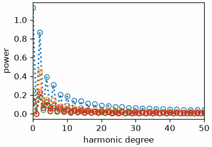
plotSpectrum draws the harmonic power spectrum of every component. The four curves show that components of one function array may have different distributions over harmonic degree.

plotSpectrum(SO3F3, lineWidth=2, figSize='small')

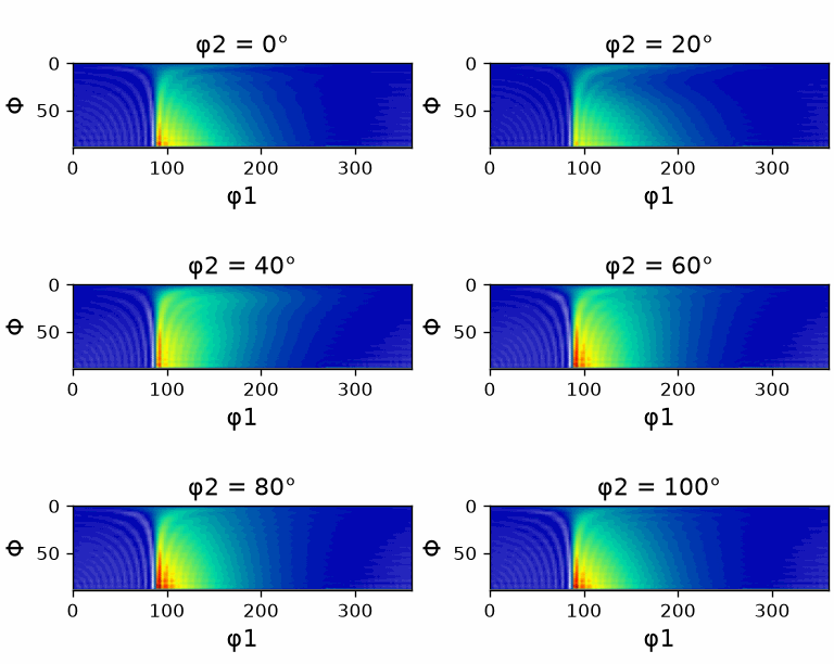
An orientation-space section plot displays only the first component of a vector-valued function, with a warning. Select and prepare a component explicitly when another component or its imaginary part is required.

with warnings.catch_warnings():
  warnings.simplefilter('ignore')
  plot(SO3F3)

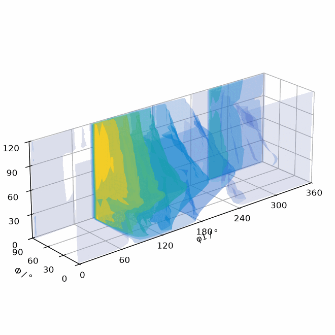
The three-dimensional plot has the same first-component restriction. The shape therefore describes the real part of the first scalar function, not the magnitude of the four-component array.

with warnings.catch_warnings():
  warnings.simplefilter('ignore')
  plot3d(SO3F3)

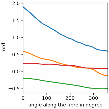
A fibre is a one-dimensional family of orientations. In contrast to the section and three-dimensional plots, plotFibre draws every component along the selected beta fibre. Here it draws the real parts, so the four curves can be compared at the same orientations.

plotFibre(SO3F3, fibre.beta(), lineWidth=2)

References

• P. J. Kostelec and D. N. Rockmore, FFTs on the rotation group, Journal of Fourier Analysis and Applications 14 (2008), 145–179, develops the Fourier representation on \(\mathrm{SO}(3)\) used for each component of an SO3FunHarmonic.

Next

Continue with Rotational Vector Fields to attach three components to specimen or crystal coordinates and account for how those vectors transform with orientation.

Technical Details

The port keeps a list of functions in NumPy’s layout: the coefficients on the last axis of fhat, where MATLAB has them on the first; a list of \(n\) functions has the shape (n,), where MATLAB’s is \(n\times 1\), and multiplying it with a \(2\times5\) array needs the column reshape(2, 1). An axis is counted from zero, MATLAB’s sum(SO3F1, 1) being sum(SO3F1, axis=0); min(f) returns the values with their positions. A function built from coefficients alone has the triclinic crystal frame on its right side where MATLAB’s has the specimen frame, so SO3F1.CS is set to that of SO3F4. Orientations take a frame at construction, so the relabelled nodes are built anew from their rotations, and the Dubna ODF is evaluated at the rotations of the triclinic nodes. The complex fourth root of \(ab\) is taken of complex numbers, as MATLAB’s power of a negative number gives. The function of the quadrature example is built from the quaternion components \(a, b, c\) of a rotation, which depend on which of \(\pm q\) represents it; the port and MATLAB choose differently, so the four functions and their spectra differ from MATLAB’s.

@article{bachmann2010mtex,
  author  = {F. Bachmann and R. Hielscher and H. Schaeben},
  title   = {Texture Analysis with MTEX - Free and Open Source Software Toolbox},
  journal = {Solid State Phenomena},
  volume  = {160},
  pages   = {63-68},
  year    = {2010},
  doi     = {10.4028/www.scientific.net/SSP.160.63},
  url     = {https://doi.org/10.4028/www.scientific.net/SSP.160.63}
}