Grain Tutorial

This tutorial starts with an EBSD map and turns its measurements into grains. It then compares pixel and grain orientations, selects grains by their properties, and previews the boundaries between two phases.

Read the EBSD tutorial first if phase maps, orientation maps, or MTEX selections are new to you. General Concepts explains how one MTEX object holds a vectorized list of measurements or grains.

The specimen is the mylonite used by Bachmann, Hielscher and Schaeben in Grain detection from 2d and 3d EBSD data. The data are courtesy of Daniel Rutte and Bret Hacker, Stanford University.

import matplotlib.pyplot as plt
import numpy as np

from mtex import *

plottingConvention.default('y↑→x')

# load the example map and display its summary
ebsd = mtexdata('mylonite')
ebsd

EBSD (y↑→x)
  size: 100 × 301 grid
  Phase  Orientations  Mineral     Color         Symmetry  Crystal reference frame
  1      3444 (28%)    Andesina    LightSkyBlue  -1        Andesina
  2      3893 (31%)    Quartz      DarkSeaGreen  -3m1      Quartz
  3      368 (2.9%)    Biotite     Goldenrod     2/m11     Biotite
  4      4781 (38%)    Orthoclase  LightCoral    12/m1     Orthoclase
  scan unit     : um
  X × Y         : [1.5e+04 → 2.4e+04] × [1020 → 3990]
  square lattice: spacing 30

# plot the phases
plot(ebsd)

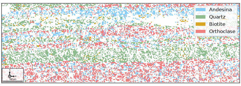
The displayed EBSD summary reports four indexed phases and the scan extent. The phase map shows quartz ribbons between mixed feldspar layers, with smaller biotite regions.

The full map is too large for the details below. We continue with a rectangle written as [xmin, ymin, width, height].

region = [19000, 1500, 4000, 1500]

# mark the selected region on the phase map
plt.gca().add_patch(plt.Rectangle(region[:2], region[2], region[3], edgecolor='black', linewidth=2, fill=False))

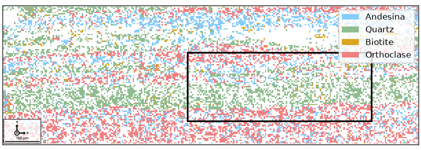
inpolygon selects the measurements inside the rectangle. Its displayed summary confirms the new extent and phase counts.

ebsdRegion = ebsd[inpolygon(ebsd, region)]
ebsdRegion

EBSD (y↑→x)
  size: 6703
  Phase  Orientations  Mineral     Color         Symmetry  Crystal reference frame
  1      578 (20%)     Andesina    LightSkyBlue  -1        Andesina
  2      1144 (40%)    Quartz      DarkSeaGreen  -3m1      Quartz
  3      58 (2%)       Biotite     Goldenrod     2/m11     Biotite
  4      1066 (37%)    Orthoclase  LightCoral    12/m1     Orthoclase
  scan unit     : um
  X × Y         : [1.902e+04 → 2.298e+04] × [1500 → 3000]
  square lattice: spacing 30

Grain reconstruction

A grain is a phase-homogeneous, spatially connected region of EBSD pixels produced by segmentation. A phase change between neighbouring pixels is always a grain boundary.

MTEX gives each measurement a spatial cell and links neighbouring cells that meet the segmentation criterion. Grain outlines follow the cell interfaces left between different linked groups.

For neighbours of the same phase, calcGrains draws a boundary when their minimum symmetry-equivalent misorientation reaches the chosen angle. The test is local between neighbours. Consequently, a gradual orientation gradient can connect two ends of one grain even when those ends differ by more than the threshold.

The 15 degree value below is an example parameter, not a universal grain definition. Grain Reconstruction explains how angle, minPixel, and alpha change the result.

# reconstruct grains and give the map a grainId property
grains = calcGrains(ebsdRegion, angle=15 * degree)

# display the grain summary
grains

grain2d (y↑→x)
  size: 998
  Phase  Grains             Mineral     Color         Symmetry  Crystal reference frame
  1      373 (578 pixels)   Andesina    LightSkyBlue  -1        Andesina
  2      189 (1144 pixels)  Quartz      DarkSeaGreen  -3m1      Quartz
  3      55 (58 pixels)     Biotite     Goldenrod     2/m11     Biotite
  4      381 (1066 pixels)  Orthoclase  LightCoral    12/m1     Orthoclase
  boundary segments: 4647, inner: 1, triple points: 1292

# plot the phase map of the selected region
plot(ebsdRegion)

# overlay the grain boundaries
hold(True)
plot(grains.boundary, lineColor='black', lineWidth=1.5)
hold(False)

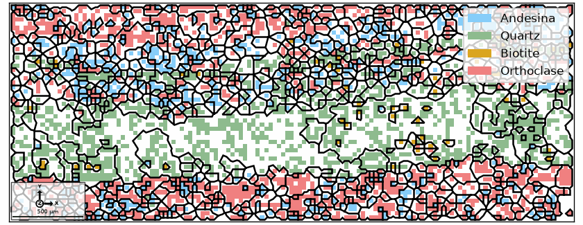
The grain summary reports a count for each phase and the number of boundary segments. In the figure, every outline follows interfaces between measurement cells rather than a hand-drawn curve. Each segment lies between neighbouring pixels assigned to different grains.

Notice the many tiny polygons. Their size makes segmentation choices and spatial resolution important before any grain-size result is reported.

Pixel orientations and grain mean orientations

A phase map says where quartz was indexed, but not how its lattice is oriented. We first colour every quartz measurement with an inverse pole figure key and draw the other phases pale.

quartzEbsd = ebsdRegion['Quartz']
quartzGrains = grains['Quartz']
ipfKey = ipfColorKey(quartzEbsd)

# plot the non-quartz grains as context
plot(grains[['Andesina', 'Biotite', 'Orthoclase']], faceAlpha=0.4)

# add the quartz measurements using one explicit colour key
hold(True)
plot(quartzEbsd, ipfKey.orientation2color(quartzEbsd.orientations))
plot(grains.boundary, lineColor='black')
legend('off')
hold(False)

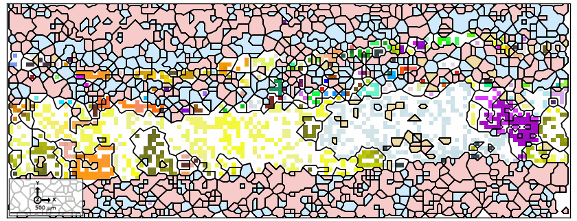
Many boundaries coincide with abrupt colour changes. Colour variation also remains inside some grains, where it may represent orientation noise or a real lattice gradient.

An IPF colour records where one specimen direction lies in the crystal. It is not a complete orientation-distance scale, so colour alone cannot validate a reconstruction. IPF Maps explains the key.

# display the colour key used for both orientation maps
plt.close('all')
plot(ipfKey)

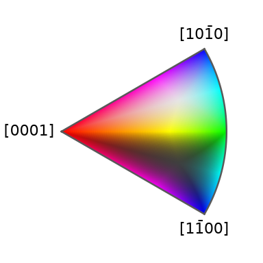
The key identifies the crystal direction represented by each colour. The same key can now colour one mean orientation per quartz grain.

# plot the non-quartz grains as context
plot(grains[['Andesina', 'Biotite', 'Orthoclase']], faceAlpha=0.4)

# colour each quartz grain by its mean orientation
hold(True)
plot(quartzGrains, ipfKey.orientation2color(quartzGrains.meanOrientation))
legend('off')
hold(False)

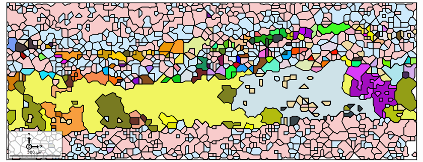
Compared with the pixel map, each quartz grain now has one flat colour. The mean suppresses intragranular variation rather than proving that the variation was noise. Orientation Parameters measures that variation explicitly.

Selecting and measuring grains

Grain properties are arrays with one value per grain. Here numPixel records the number of measurements assigned to a grain, while area measures its sectional area in the scan unit.

The next selection keeps quartz grains with at least ten measurements and removes grains cut by the edge of the map. The value ten only illustrates a logical selection; it is not a recommended quality criterion.

selectedQuartz = grains['Quartz', (grains.numPixel >= 10) & ~grains.isBoundary]
selectedQuartz

grain2d (y↑→x)
  size: 13
  Phase  Grains           Mineral  Color         Symmetry  Crystal reference frame
  2      13 (451 pixels)  Quartz   DarkSeaGreen  -3m1      Quartz
  boundary segments: 634, inner: 0, triple points: 133
        Id   Phase  Pixels        meanRotation         GOS
       257       2      51      (171°,32°,65°)      0.0548
       279       2      23      (3°,121°,115°)      0.0378
       281       2      37      (1°,121°,113°)      0.0253
       308       2      17      (2°,121°,117°)      0.0164
       309       2     203     (165°,112°,44°)      0.0177
       320       2      10       (176°,60°,2°)      0.0183
       325       2      33     (161°,117°,88°)     0.00927
       347       2      10      (1°,121°,114°)      0.0124
       354       2      22     (161°,117°,87°)      0.0102
       364       2      10     (161°,118°,27°)      0.0119
       374       2      11       (1°,152°,53°)      0.0503
       540       2      12        (3°,148°,3°)      0.0286
       620       2      12      (153°,117°,8°)      0.0574

The displayed grain2d summary reports what the selection retained. Because calcGrains gave ebsdRegion a grainId property, the selection also leads back to its measurements.

selectedMeasurements = ebsdRegion[selectedQuartz]
selectedMeasurements

EBSD (y↑→x)
  size: 451
  Phase  Orientations  Mineral  Color         Symmetry  Crystal reference frame
  2      451 (100%)    Quartz   DarkSeaGreen  -3m1      Quartz
  properties    : grainId
  scan unit     : um
  X × Y         : [1.917e+04 → 2.283e+04] × [1770 → 2640]
  square lattice: spacing 30

The measurement summary contains only quartz pixels assigned to the selected grains. The grains themselves can be coloured by area.

plt.close('all')
plot(grains, faceColor='lightgray', faceAlpha=0.3)
hold(True)
plot(selectedQuartz, selectedQuartz.area)
hold(False)
legend('off')
mtexColorbar(title='sectional grain area')

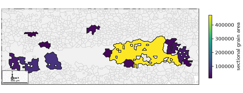
The coloured regions are the selected interior quartz grains, and their colour represents area rather than orientation. Removing edge grains avoids treating a clipped grain as if its full section had been measured.

A two-dimensional section does not directly give three-dimensional grain volume. Step size, segmentation settings, and the treatment of small or notIndexed regions must also be fixed before specimens are compared. notIndexed is the phase for measurements whose diffraction patterns could not be indexed. Shape Parameters develops these measurements.

Boundaries between two phases

A phase boundary is not a separate type of object. It is a grain boundary whose two neighbouring grains differ in phase, selected here by two names.

Every segment between andesina and orthoclase carries a misorientation. Its angle is the minimum over the symmetries of both phases.

plt.close('all')

# select the boundary segments between two phases and display their summary
aoBoundary = grains.boundary['Andesina', 'Orthoclase']
aoBoundary

grainBoundary (y↑→x)
  size: 1176 segments, 673 chains
  segments    length  mineral 1   mineral 2
      1176  40027 µm   Andesina  Orthoclase

# store one angle per boundary segment in radians
boundaryAngle = aoBoundary.misorientation.angle()

# highlight an illustrative part of the angular range
plot(grains, faceAlpha=0.4)
hold(True)
plot(aoBoundary[boundaryAngle > 160 * degree], lineWidth=2, lineColor='red')
hold(False)

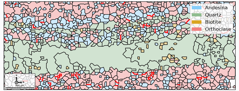
The red traces are the segments above the illustrative 160 degree filter. This filter is applied after reconstruction and did not define the grains. A phase change already made every andesina to orthoclase contact a boundary.

One physical interface is represented by many connected segments. A segment count is therefore neither a count of interfaces nor a set of independent observations.

Weighting by segLength gives longer interfaces proportionally more influence. It avoids weighting every tessellation segment equally.

# bin the angles and sum the segment lengths falling into each bin
edges = np.histogram_bin_edges(boundaryAngle / degree, 'auto')
histogram(boundaryAngle / degree, edges, weights=aoBoundary.segLength)
xlabel('minimum misorientation angle (degrees)')
ylabel('boundary trace length')
plt.title('Andesina to orthoclase orientation relationships')

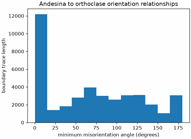
Notice how the traced boundary length is distributed across the angular range. This plot is descriptive, not evidence that either phase pair is related more often than chance.

Such a claim needs a stated reference distribution and consistent sampling weights. Continue with the grain boundary tutorial, then Boundary Misorientations and Misorientation Distribution Functions.

Next

Selecting Grains covers selection by position, phase, property, and orientation. Grain Plots and Shape Parameters develop grain measurements.

Grain mean orientations can also be used for pole figures and ODFs. Giving every grain one vote answers a different question from weighting pixels or grain area; ODF Estimation explains the choice.

For your own data, read Reference Frame before interpreting orientation-dependent results. The reconstructed regions continue into the Grains chapter, while their interfaces continue into Grain Boundaries.

Further reading

• F. Bachmann, R. Hielscher and H. Schaeben, Grain detection from 2d and 3d EBSD data - Specification of the MTEX algorithm, Ultramicroscopy 111 (2011), 1720-1733.
• F.J. Humphreys, Grain and subgrain characterisation by electron backscatter diffraction, Journal of Materials Science 36 (2001), 3833-3854.
• A.J. Schwartz et al., editors, Electron Backscatter Diffraction in Materials Science, 2nd ed., Springer, 2009.
• ISO 13067:2020 specifies EBSD procedures for average grain size from two-dimensional sections and warns that highly deformed specimens require care.
• ASTM E2627-13(2019) covers EBSD grain-size measurement in fully recrystallized polycrystals. That scope does not include the deformed mylonite used on this page.

Technical Details

The mylonite file lists only the indexed measurements, so the port reads it onto its 100 x 301 grid and marks the missing cells as padding. The displays count, and the selections return, only the measurements; the size of ebsdRegion is that of its cells. The reconstruction gives 373 andesina grains for MATLAB’s 371 and 4647 boundary segments for 4527, the other phases and the 13 selected quartz grains with their 451 measurements as MATLAB’s; 1176 andesina to orthoclase segments for 1180.

MATLAB’s histcounts chooses its bins by its own rule (20 degree bins here); the page takes NumPy’s 'auto' edges, 15 degree bins, and weights them by segLength in one call, where MATLAB sums the lengths with accumarray.

@article{bachmann2010mtex,
  author  = {F. Bachmann and R. Hielscher and H. Schaeben},
  title   = {Texture Analysis with MTEX - Free and Open Source Software Toolbox},
  journal = {Solid State Phenomena},
  volume  = {160},
  pages   = {63-68},
  year    = {2010},
  doi     = {10.4028/www.scientific.net/SSP.160.63},
  url     = {https://doi.org/10.4028/www.scientific.net/SSP.160.63}
}