EBSD3.calcGrains

the grains of a map, the pixels joined across every boundary the criterion keeps; MATLAB’s grain reconstruction from 2d and 3d EBSD data

Syntax

grains = calcGrains(ebsd)

grains = calcGrains(ebsd, angle=10*degree, minPixel=5, alpha=3.7)

grains = calcGrains(ebsd, angle=[10*degree, 2*degree])

grains = calcGrains(ebsd, angle=[[10*degree], [5*degree]])

grains = calcGrains(ebsd, criterion=gbcAngle(10*degree, byPhase={'Enstatite': 5*degree}))

grains = calcGrains(ebsd, criterion=gbcSoft(10*degree, 2*degree), mcl=(1.4, 4))

grains = calcGrains(ebsd, fmc=1.5, minPixel=10)

grains = calcGrains(ebsd, grainId=True)

Description

Two neighbouring pixels belong to one grain when the misorientation between them stays below the threshold angle, and a grain is a connected set of such pixels. The angle takes these forms:

• one angle: the threshold of every phase.
• a pair [high, low]: the boundaries above high separate the grains, those between low and high stay inside them as low angle boundaries, grains.innerBoundary.
• a list of other than two entries, or of lists: an angle or a pair per indexed phase or per entry of ebsd.CSList, as MATLAB’s cell {a1, a2, a3}; two phases take [[a1], [a2]].

Any other rule, a soft threshold included, is a grainBoundaryCriterion.

A map of the plane is divided into cells around its pixels, a Voronoi decomposition bounded by alpha. A not indexed region narrower than 2 alpha pixel spacings is filled by the grains around it, a wider one becomes a notIndexed grain.

The map is changed: it keeps the grain ids, the pixels the minPixel cull drops and the notIndexed pixels the grains absorb, so MATLAB’s second output is the map passed. Run on ebsd.copy() to keep the map as it was.

Input

Keywords

Output

Example

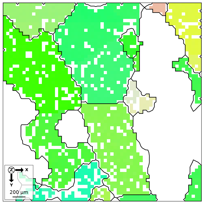
Reconstruct grains in the small Forsterite sample and overlay their boundaries on an orientation map. The first call downloads and caches the sample file; later calls reuse it.

import numpy as np
import matplotlib.pyplot as plt
from mtex import mtexdata, calcGrains, degree, plot, hold

ebsd = mtexdata('small', verbose=False)['Forsterite']
grains = calcGrains(ebsd, angle=10*degree, minPixel=5)
print('Grains:', grains.size)
print('Grain ids assigned to pixels:', np.unique(ebsd.grainId)[:8])
plot(ebsd, ebsd.orientations)
hold(True)
plot(grains.boundary, lineColor='black', lineWidth=1.5)
hold(False)
plt.show()

The threshold is illustrative. calcGrains writes grain ids into ebsd and may change pixels when minPixel removes small grains; call it on ebsd.copy() when the original map is needed.

Grains: 15
Grain ids assigned to pixels: [0 1 2 3 4 5 6 7]

References

• F. Bachmann, R. Hielscher, H. Schaeben, Grain detection from 2d and 3d EBSD data - Specification of the MTEX algorithm, Ultramicroscopy 111 (2011) 1720-1733
• C. McMahon, B. Soe, A. Loeb, A. Vemulkar, M. Ferry, L. Bassman, Boundary identification in EBSD data with a generalization of fast multiscale clustering, Ultramicroscopy 133 (2013) 16-25

See also

GrainReconstruction, GrainReconstructionAdvanced, GrainReconstructionMCL, gbcAngle, grain2d.merge, smoothBoundary

Used on

CrystalShapes, OrientationFundamentalRegion, EBSD3Analysis, EBSD3Plotting, Grains3DBoundaries, Grains3DReconstruction, Grains3DSmoothing, EBSD2ODF, EBSDDenoising, EBSDFilling, EBSDGROD, EBSDGrid

MATLAB’s EBSD3.calcGrains

@article{bachmann2010mtex,
  author  = {F. Bachmann and R. Hielscher and H. Schaeben},
  title   = {Texture Analysis with MTEX - Free and Open Source Software Toolbox},
  journal = {Solid State Phenomena},
  volume  = {160},
  pages   = {63-68},
  year    = {2010},
  doi     = {10.4028/www.scientific.net/SSP.160.63},
  url     = {https://doi.org/10.4028/www.scientific.net/SSP.160.63}
}