Smoothing Three-Dimensional Grain Boundaries

Grains reconstructed from voxel data have a boundary that follows the voxel faces. Every face normal points along one of the three axes, so a boundary normal distribution or a curvature computed from it measures the grid, not the specimen. This page coarsens the voxel surface, smooths it, and measures the price in grain volume. The aim is a surface suitable for quantitative analysis, not simply a smoother-looking picture.

import matplotlib.pyplot as plt
import numpy as np

from mtex import *

plottingConvention.default('y↑→x')
how2plot = plottingConvention.default3D

fname = mtexdatafile('SmallIN100')
ebsd = EBSD3.load(fname)
grains = calcGrains(ebsd, angle=5 * degree)
print(grains)

grain3d (y↑→x)
  Phase  Grains              Mineral  Color         Symmetry  Crystal reference frame
  1      812 (volume 15625)  unknown  LightSkyBlue  432       unknown
  boundary faces: 757562

The boundary network is stratified

A boundary face separates two grains. Along a triple line three grains meet, at a quadruple point four. nodeType counts the grains at every vertex and adds 10 on the outer hull of the measured volume, where a vertex inside a single grain also occurs. These are counts of mesh vertices, so they depend on resolution; they are not counts of complete triple lines or physical quadruple points.

t = grains.boundary.nodeType()
n = np.bincount(t[t > 0])
print(np.column_stack([np.flatnonzero(n), n[n > 0]]))

[[     2 241422]
 [     3  41328]
 [     4   3806]
 [     5    167]
 [     6      4]
 [    11  46985]
 [    12  11912]
 [    13   1078]
 [    14     27]]

A junction must not be averaged with the interior of a face, which is why the smoothing below treats each stratum in turn.

Coarsen first

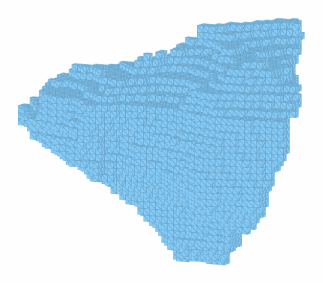
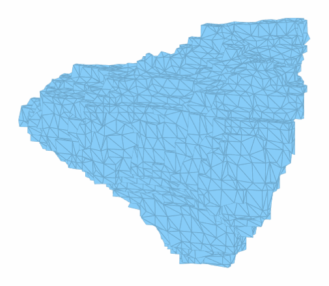
reduceBoundary merges the vertices of each cell of twice the voxel size into one. Clustering distinguishes the grains meeting at a vertex and the faces of the hull, preserving their junction structure where the coarsened mesh remains resolved. The centroid of a cluster already averages the voxel steps; the flag quadric=True puts the vertex where the faces around it are best approximated instead, which keeps flat boundaries flat.

grainsC = reduceBoundary(grains, 2, quadric=True)
print(grainsC)

grain3d (y↑→x)
  Phase  Grains              Mineral  Color         Symmetry  Crystal reference frame
  1      812 (volume 15625)  unknown  LightSkyBlue  432       unknown
  boundary faces: 289348

Check how many faces remain and whether very small grains have lost their enclosing surface. Coarsening can collapse a grain below its cell size; this matters when the fine-grain population is part of the question.

print([len(grains.boundary), len(grainsC.boundary)])
print(np.count_nonzero(grainsC.volume <= 0))

[757562, 289348]
6

The largest grain makes the geometric change easy to see.

id = int(np.argmax(grains.volume))
plot(grains[id], micronbar='off', edgeAlpha=0.2)
setCamera(how2plot)

plot(grainsC[id], micronbar='off', edgeAlpha=0.2)
setCamera(how2plot)

Smooth

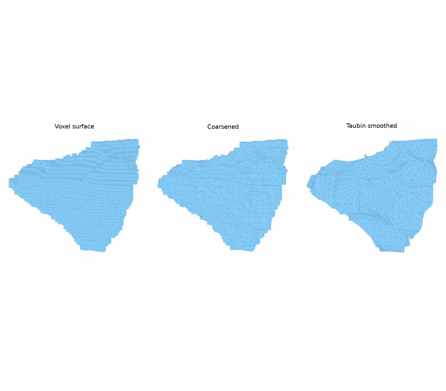
smoothBoundary moves the vertices and nothing else. Quadruple points and the hull stay fixed, every triple line is smoothed as a curve between its quadruple points, and every boundary face as a surface between its triple lines. The filters are the ones of the two-dimensional grain smoothing: laplaceFilter shrinks each grain a little per iteration, taubinFilter keeps the volumes approximately, curvatureFilter solves for a smoothing length in one step.

grainsS = smoothBoundary(grainsC, taubinFilter(20))
newMtexFigure(layout=[1, 3], figSize='large')
plot(grains[id], micronbar='off', edgeAlpha=0.2)
setCamera(how2plot)
mtexTitle('Voxel surface')
nextAxis()
plot(grainsC[id], micronbar='off', edgeAlpha=0.2)
setCamera(how2plot)
mtexTitle('Coarsened')
nextAxis()
plot(grainsS[id], micronbar='off', edgeAlpha=0.2)
setCamera(how2plot)
mtexTitle('Taubin smoothed')

3D views: 1, 2, 3

Triple lines remain shared by the same grains, but their vertices may move. Add fixTripleLines=True to hold them fixed during smoothing. Keeping the outer hull fixed conserves the enclosed total volume for a valid mesh; it does not conserve each grain’s volume.

Compare Laplace and Taubin smoothing from the same coarsened mesh. Include the coarsened result separately so its contribution is visible.

grainsL = smoothBoundary(grainsC, laplaceFilter(20))
vol = np.column_stack([grains.volume, grainsC.volume, grainsL.volume, grainsS.volume])
print(vol.sum(axis=0))

[15625. 15625. 15625. 15625.]

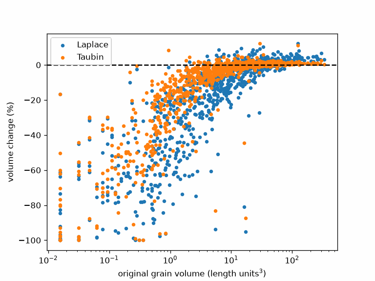
Relative volume change reveals whether the surface treatment affects the fine grains more strongly. The three columns below correspond to coarsening, coarsening plus Laplace, and coarsening plus Taubin.

relativeChange = 100 * (vol[:, 1:] - vol[:, :1]) / vol[:, :1]
print(np.median(np.abs(relativeChange), axis=0))

plt.figure()
plt.scatter(vol[:, 0], relativeChange[:, 1], 12, label='Laplace')
plt.scatter(vol[:, 0], relativeChange[:, 2], 12, label='Taubin')
plt.axhline(0, color='k', linestyle='--')
plt.xscale('log')
plt.xlabel('original grain volume (length units$^3$)')
plt.ylabel('volume change (%)')
plt.legend(loc='best')

[ 0.6447 11.961   3.3128]

The option maxDisplacement limits each coordinate change relative to the mesh entering the smoothing step. It does not undo displacement or a collapsed grain from coarsening. For example, half the smallest voxel spacing gives a bound tied to measurement resolution:

grainsBounded = smoothBoundary(grainsC, taubinFilter(20),
                               maxDisplacement=0.5 * min(ebsd.dx, ebsd.dy, ebsd.dz))

The scheme scheme='coupled' smooths all movable vertices together instead of treating triple lines before face interiors. Compare its geometric effect if junction positions are central to the analysis.

What the smoothing changes downstream

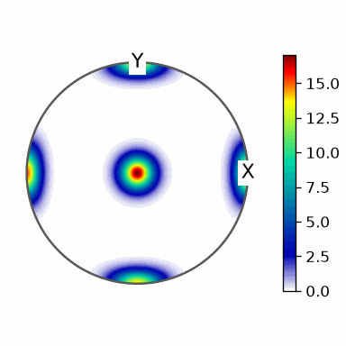
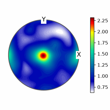
The boundary normal distribution of the voxel surface has all its weight on the three axes. After smoothing the normals spread over the sphere.

gB = grains.boundary
gB = gB[np.all(gB.grainId > 0, axis=1)]
plot(calcGBND(gB), upper=True)
mtexColorbar()

gBS = grainsS.boundary
gBS = gBS[np.all(gBS.grainId > 0, axis=1)]
plot(calcGBND(gBS), upper=True)
mtexColorbar()

Refine

refineBoundary splits every edge at its midpoint and every face into four. No vertex moves, so volumes, areas and the grains a face separates are inherited exactly. Refinement increases mesh density, for instance before a filter with a short smoothing length. It adds no measurement information and cannot recover a feature removed by coarsening.

grainsR = refineBoundary(grainsS)
print([len(grainsS.boundary), len(grainsR.boundary)])

[289348, 1157392]

Choose the treatment for the quantity being measured

Volume, area and normal distributions need different levels of geometric fidelity. The area change below complements the volume comparison: a small change in volume can accompany a large decrease in staircase area.

surfaceArea = np.array([grains.surface().sum(), grainsC.surface().sum(), grainsL.surface().sum(), grainsS.surface().sum()])
print(100 * (surfaceArea / surfaceArea[0] - 1))

[  0.     -15.0252 -32.9219 -31.0261]

Here the sum counts shared interfaces twice, consistently for all four meshes. For a physical internal area per volume, count each interface once as on the Boundary Network page. Repeat the comparison with a smaller coarsening factor or fewer filter iterations: a conclusion about morphology should survive reasonable choices near the voxel resolution. A smooth mesh alone does not establish a resolved curvature or remove uncertainty from missing orientations.

Function reference

References

• S. Maddali, S. Ta’asan, R. M. Suter, Topology-faithful nonparametric estimation and tracking of bulk interface networks, Computational Materials Science 125 (2016), 328-340, the hierarchical treatment of quadruple points, triple lines and faces.
• G. Taubin, A signal processing approach to fair surface design, SIGGRAPH 1995, the λ|μ filter without shrinkage.
• M. Desbrun, M. Meyer, P. Schröder, A. H. Barr, Implicit fairing of irregular meshes using diffusion and curvature flow, SIGGRAPH 1999, smoothing as one linear solve.
• J. Rossignac, P. Borrel, Multi-resolution 3D approximations for rendering complex scenes, Modeling in Computer Graphics, Springer 1993, vertex clustering.
• P. Lindstrom, Out-of-core simplification of large polygonal models, SIGGRAPH 2000, the quadric placement of a cluster.
• S. F. F. Gibson, Constrained elastic surface nets, MICCAI 1998, the bound on the displacement.
• M. A. Groeber, M. A. Jackson, DREAM.3D: a digital representation environment for the analysis of microstructure in 3D, Integrating Materials and Manufacturing Innovation 3 (2014), the node types and the coupled scheme.

Next

Continue with Boundary Network to measure interface area and inspect junctions. Properties measures the enclosed grains, and Boundary Normal Distribution develops the analysis of their surface normals.

Technical details

MATLAB’s flags 'quadric', 'fixTripleLines', 'coupled' are the keywords quadric=True, fixTripleLines=True, scheme='coupled'; nodeType is a method of the boundary, and the largest grain’s position counts from 0.

@article{bachmann2010mtex,
  author  = {F. Bachmann and R. Hielscher and H. Schaeben},
  title   = {Texture Analysis with MTEX - Free and Open Source Software Toolbox},
  journal = {Solid State Phenomena},
  volume  = {160},
  pages   = {63-68},
  year    = {2010},
  doi     = {10.4028/www.scientific.net/SSP.160.63},
  url     = {https://doi.org/10.4028/www.scientific.net/SSP.160.63}
}