The Three-Dimensional Boundary Network

The boundary of a set of three-dimensional grains is one surface mesh for the whole volume. Every face separates two grains and, when the grains were reconstructed from voxels, knows the two voxels it separates. Along the edges where three grains meet run the triple lines, and where four grains meet sits a quadruple point. These contacts constrain grain growth and provide possible paths for intergranular transport or damage. This page measures how much interface is present and shows how the junctions connect it, using the IN100 volume of the reconstruction page.

import numpy as np

from mtex import *

plottingConvention.default('y↑→x')
how2plot = plottingConvention.default3D

fname = mtexdatafile('SmallIN100')
ebsd = EBSD3.load(fname)
grains = calcGrains(ebsd, angle=5 * degree)
gB = grains.boundary
print(gB)

grain3Boundary
  faces   : 757562 triangles (637562 between grains, 120000 on the outside)
  vertices: 346729

One face, two grains, two voxels

A face is a triangle, two per voxel face. grainId holds the two grains it separates, with the face normal pointing from the first into the second. ebsdId holds the two voxels on either side, and misorientation the misorientation between their orientations, computed from the voxels rather than from the grain means. Faces on the outer hull of this voxel reconstruction have a zero in the second column of both. In a general imported mesh the zero can occur on either side, so test both columns.

print(np.hstack([gB.grainId[:5], gB.ebsdId[:5]]))

[[   150     56 200000 210000]
 [   150     56 200000 210000]
 [    56    137 250000 260000]
 [    56    137 250000 260000]
 [   137     51 340000 350000]]

Count area, not triangles: refining a face changes its mesh count without adding any physical interface. The following fractions distinguish the measurement hull from contacts between indexed grains.

faceArea = gB.area
isHull = np.any(gB.grainId == 0, axis=1)
isIndexed = np.all(gB.isIndexed, axis=1) & ~isHull
print(np.r_[faceArea[isHull].sum(), faceArea[isIndexed].sum()] / faceArea.sum())

[0.1584 0.8416]

Select faces

A boundary is selected like a list: by the grains at its sides, by phase, or by any property of the faces. The faces of one grain, the faces between two grains, and the faces above a misorientation angle are three common selections.

largestIndex = int(np.argmax(grains.volume))
id = grains.id[largestIndex]
gBid = gB[np.any(gB.grainId == id, axis=1)]
neighbours = np.setdiff1d(np.unique(gBid.grainId), [0, id])
gBpair = gB[np.any(gB.grainId == id, axis=1) & np.any(gB.grainId == neighbours[0], axis=1)]
gBhigh = gB[(gB.misorientation.angle() > 30 * degree) & np.all(gB.grainId > 0, axis=1)]

print([len(gBid), len(gBpair), len(gBhigh)])

[16524, 300, 547682]

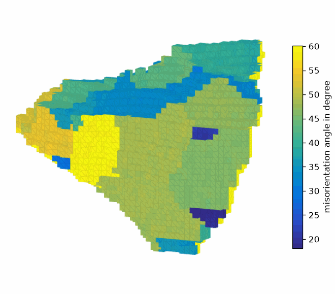
The largest grain, with its faces coloured by the misorientation angle across them. Each triangle has one value, but the values may vary over a contact between the same two grains: they come from the local voxel orientations. Missing orientations and the measurement hull do not supply a meaningful misorientation angle.

plot(gBid, gBid.misorientation.angle() / degree, edgeAlpha=0.1, micronbar='off')
setCamera(how2plot)
mtexColorbar(title='misorientation angle in degree')

Edges, triple lines and quadruple points

edges lists every edge once and tells for each face which three edges bound it. An edge on two faces lies inside a boundary face, an edge on three or more faces on a triple line. nodeType counts the grains at every vertex: 2 inside a face, 3 on a triple line, 4 at a quadruple point, and 10 more for a vertex on the outer hull.

E, F2E = gB.edges()
isTripleLine = np.bincount(F2E.reshape(-1), minlength=len(E)) >= 3
t = gB.nodeType()

print([len(E), np.count_nonzero(isTripleLine), np.count_nonzero(t % 10 == 3), np.count_nonzero(t % 10 >= 4)])

[1103992, 62789, 42406, 4004]

The triple lines of the largest grain, drawn over its faces. Every line is where a neighbour ends and the next one begins, and the lines meet at the quadruple points.

V = gB.allV
onGrain = np.zeros(len(V), dtype=bool)
onGrain[gBid.F.reshape(-1)] = True
onGrainEdge = np.zeros(len(E), dtype=bool)
onGrainEdge[F2E[np.any(gB.grainId == id, axis=1)]] = True
Eid = E[isTripleLine & onGrainEdge]
nan = np.full(len(Eid), np.nan)
X, Y, Z = (np.column_stack([V[Eid[:, 0], k], V[Eid[:, 1], k], nan]).reshape(-1) for k in range(3))

plot(gBid, faceColor=[0.85, 0.85, 0.85], edgeAlpha=0.1, micronbar='off')
hold(True)
line(X, Y, Z, color='r', lineWidth=1.5)
isQuad = (t % 10 >= 4) & onGrain
plot(vector3d(V[isQuad]), color='b', markerSize=5.5)
hold(False)
setCamera(how2plot)

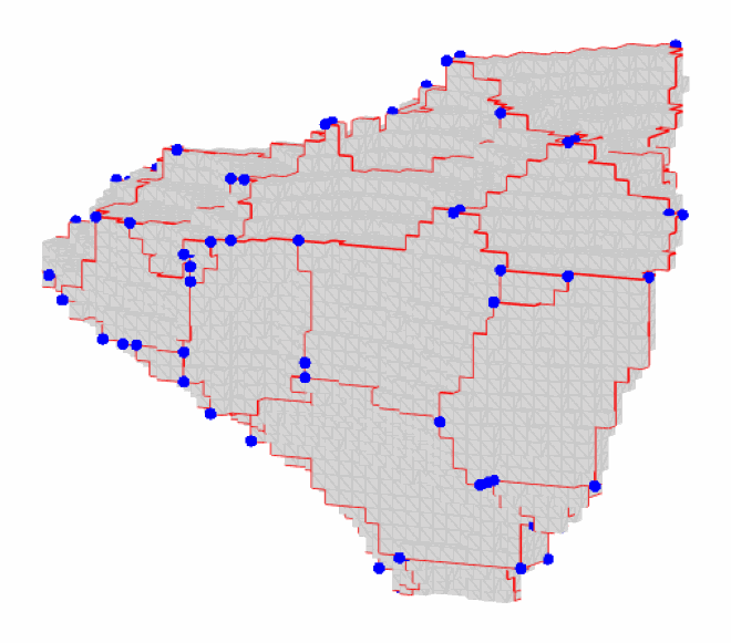
The counts describe mesh vertices, not numbers of physical junctions. A triple line has many vertices, and voxel corners can join more than four grains. Types above 10 identify junctions on the measurement hull.

n = np.bincount(t[t > 0])
print(np.column_stack([np.flatnonzero(n), n[n > 0]]))

[[     2 241422]
 [     3  41328]
 [     4   3806]
 [     5    167]
 [     6      4]
 [    11  46985]
 [    12  11912]
 [    13   1078]
 [    14     27]]

From faces to the boundary character

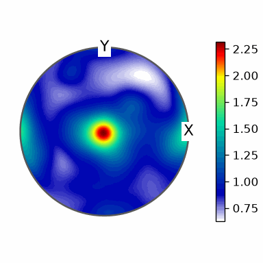
Each face carries all five parameters of a grain boundary: the misorientation of the two grains and the normal of the face. The normals of the voxel surface point along the axes, so the surface has to be smoothed first, see Smoothing, before the boundary normal distribution or the boundary character distribution reads anything but the voxel grid.

grainsS = smoothBoundary(reduceBoundary(grains, 2, quadric=True), taubinFilter(20))
gBS = grainsS.boundary['indexed']

plot(calcGBND(gBS), upper=True)
mtexColorbar()

How much internal boundary is there per unit volume?

Boundary area per specimen volume is a useful geometric input when comparing interfacial storage or transport between microstructures. Each shared face appears once in grains.boundary. Summing grains.surface() instead would count an internal interface twice and include the hull.

internal = np.all(grainsS.boundary.grainId > 0, axis=1)
internalArea = grainsS.boundary[internal].area.sum()
boundaryAreaDensity = internalArea / grainsS.volume.sum()
print(boundaryAreaDensity)

0.8422676432793769

The unit is inverse length. This value uses all internal contacts and the full reconstructed volume. To report only indexed grain boundaries, use grainsS.boundary['indexed'] and state the corresponding volume denominator.

What fraction of indexed boundary area has a low angle?

Use a stated angle threshold and weight by face area. This describes the local misorientation stored on the reconstructed faces, rather than a count of low-angle grain pairs. After coarsening, the retained faces carry inherited misorientations; remeasure from the original data if local orientation gradients are the quantity of interest.

angleLimit = 15 * degree
lowAngle = gBS.misorientation.angle() < angleLimit
lowAngleAreaFraction = gBS[lowAngle].area.sum() / gBS.area.sum()
print(lowAngleAreaFraction)

0.02921802537286299

A low-angle fraction alone does not establish a connected boundary path. Connectivity also requires the grain pairs and junction network. Likewise, the specimen-frame normal distribution above describes preferred interface inclinations, not preferred crystallographic planes. For one selected phase, calcGBND(gBS, grainsS['phase name']) transforms normals into the crystal frame; see Boundary Normal Distribution.

Function reference

References

• G. S. Rohrer, Measuring and interpreting the structure of grain-boundary networks, Journal of the American Ceramic Society 94 (2011), 633-646, the five parameter description of a boundary and its distribution from a triangle mesh.
• M. A. Groeber, M. A. Jackson, DREAM.3D: a digital representation environment for the analysis of microstructure in 3D, Integrating Materials and Manufacturing Innovation 3 (2014), the node types of the boundary network.

Next

Continue with Neper Interface to construct a synthetic comparison, or go to Properties to measure grain size and shape. Smoothing explains the geometric treatment used before the surface measurements above.

Technical details

calcGrains alters the volume it is given (the grain ids stay on it), so MATLAB’s [grains, ebsd] = calcGrains(ebsd, ...) is grains = calcGrains(ebsd, ...). edges and nodeType are methods of the boundary and accumarray is np.bincount. The grain ids count from 1 as MATLAB’s, 0 standing for the outside; ebsdId counts the voxels from 0 in the port’s array order, -1 standing for the outside, as for every map of the port.

@article{bachmann2010mtex,
  author  = {F. Bachmann and R. Hielscher and H. Schaeben},
  title   = {Texture Analysis with MTEX - Free and Open Source Software Toolbox},
  journal = {Solid State Phenomena},
  volume  = {160},
  pages   = {63-68},
  year    = {2010},
  doi     = {10.4028/www.scientific.net/SSP.160.63},
  url     = {https://doi.org/10.4028/www.scientific.net/SSP.160.63}
}