Neper Interface

Neper is an open-source package developed by Romain Quey for generating and meshing polycrystals. MTEX can configure a Neper tessellation, run it, and load the result as a grain3d collection. A synthetic volume lets us vary morphology and texture independently, test how sectioning changes a measured distribution, or prepare grain geometry for a simulation. Three-Dimensional Grains defines that representation and introduces selection and sectioning.

A planar section is useful when the three-dimensional microstructure must be compared with a two-dimensional map. It is not required for analysing the original grain3d collection.

import os
import tempfile

import matplotlib.pyplot as plt
import numpy as np

from mtex import *

plottingConvention.default('y↑→x')

Check the external program

Install Neper separately and make its executable available on the system path. Its documentation gives platform-specific installation instructions. The preference neperCommand names another executable.

The check below keeps this page executable on systems without Neper. In that case, the simulation section loads a bundled tessellation explicitly. This avoids mistaking an old output file for a successful new simulation.

hasNeper = neper.init().available()

Choose files and geometry

neper.init returns the interface object. By default, Neper works in os.path.join(tempfile.gettempdir(), 'neper'). Keeping generated files under the temporary directory prevents a documentation run from overwriting a project tessellation.

The default three-dimensional base name is allgrains, and the default two-dimensional base name is 2dslice. Neper adds .tess and .ori; three-dimensional output may also include .stpoly. Assign filePath, fileName3d, or fileName2d when these defaults are unsuitable.

if hasNeper:
  neper = neper.init()
  neper.filePath = os.path.join(tempfile.gettempdir(), 'mtex-neper-doc')
  neper.fileName3d = 'my100grains'
  neper.fileName2d = 'my100GrSlice'

For example, an existing project directory could be selected with

neper.filePath = 'C:/Users/user/Documents/work/MtexWork/neper'

Neper coordinates set relative lengths; choose their physical scale for the intended material or simulation. The geometry property controls the outer domain. Its default is "cube(1,1,1)". Cuboids use "cube(x,y,z)"; cylinders use "cylinder(h,d,numFaces)"; spheres use "sphere(d,numFaces)".

if hasNeper:
  neper.geometry = "cube(4,4,2)"

Control repeatability and morphology

Neper uses the integer id as the seed for the initial seed positions. Reusing it makes the initial tessellation repeatable. The default is 1.

The morpho string sets the target cell morphology. The default 'graingrowth' is an alias for the lognormal equivalent-diameter and sphericity distributions below. Neper documents further choices under morphology options.

if hasNeper:
  neper.id = 529
  neper.morpho = 'diameq:lognormal(1,0.35),1-sphericity:lognormal(0.145,0.03)'

Simulate a textured microstructure

simulateGrains accepts either an orientation distribution function (ODF) and a grain count, or a list of orientations. For a list, its length determines the grain count. With silent=True Neper’s console output goes to neper.log in filePath. Both the generated grains and the imported example use the ODF’s trigonal quartz symmetry, also used on the Properties and Operations pages.

# the Dubna ODF has trigonal quartz symmetry
odf = SO3Fun.dubna()
numGrains = 100

if hasNeper:
  grains = neper.simulateGrains(numGrains, odf, verbose=False)
else:
  tessFile = mtexdatafile('my100grains')[0]
  grains = grain3d.load(tessFile, CS=odf.CS)
print(grains)

grain3d (y↑→x)
  Phase  Grains           Mineral  Color         Symmetry  Crystal reference frame
  1      100 (volume 32)  Quartz   LightSkyBlue  321       Quartz
  boundary faces: 643

To prescribe every orientation rather than sample the ODF internally, use

ori = odf.discreteSample(numGrains)
grains = neper.simulateGrains(ori, silent=True)

The summary confirms that the result is a three-dimensional grain collection. The fallback is an existing example, not a realization of the settings above: it retains its stored geometry and orientations. The ODF controls grain orientations, not a boundary-normal distribution or a constitutive law.

plot(grains, grains.meanOrientation, micronbar='off', edgeAlpha=0.1)
how2plot = plottingConvention.default3D
setCamera(how2plot)

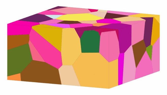
The colours encode one mean orientation per polyhedral grain. The outer envelope follows the cuboid selected by the simulation that created this tessellation.

Check the generated size distribution

A morphology string specifies a target, not the measured outcome of a finite tessellation. Check the resulting equivalent-sphere diameters before treating the volume as a representative microstructure. Normalizing by the mean separates the spread from the chosen length scale.

diameter = (6 * grains.volume / np.pi) ** (1 / 3)
newMtexFigure()
histogram(diameter / diameter.mean(), 15)
plt.xlabel('equivalent-sphere diameter / mean diameter')
plt.ylabel('number of grains')

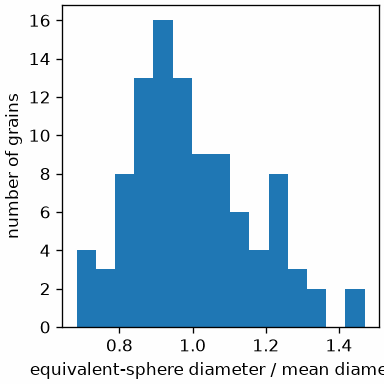
Use several seeds and, when needed, more grains to assess sampling variability. A prescribed list of orientations gives one orientation per grain; unequal grain volumes mean its volume-weighted texture can differ from the number-weighted orientation sample.

Compare planar sections

The earlier sectioning example defines slice. A slice normal and either a point in the plane or its signed distance from the origin specify the cutting plane. Here all three sections pass through the centre of the collection.

N = [vector3d(0, 0, 1), vector3d(1, -1, 0), vector3d(2, 2, 4)]
A = grains.midPoint

grains001 = grains.slice(N[0], A)
grains1_10 = grains.slice(N[1], A)
grains224 = grains.slice(N[2], A)
print(grains224)

newMtexFigure(layout=[1, 3], figSize='large')
plot(grains001, grains001.meanOrientation, micronbar='off')
mtexTitle('normal || specimen z')
nextAxis()
plot(grains1_10, grains1_10.meanOrientation, micronbar='off')
mtexTitle('normal || (1,-1,0)')
nextAxis()
plot(grains224, grains224.meanOrientation, micronbar='off')
mtexTitle('normal || (2,2,4)')

grain2d (y↑→x)
  size: 49
  Phase  Grains          Mineral  Color         Symmetry  Crystal reference frame
  1      49 (49 pixels)  Quartz   LightSkyBlue  321       Quartz
  boundary segments: 150, inner: 0, triple points: 72
  properties       : Id3d

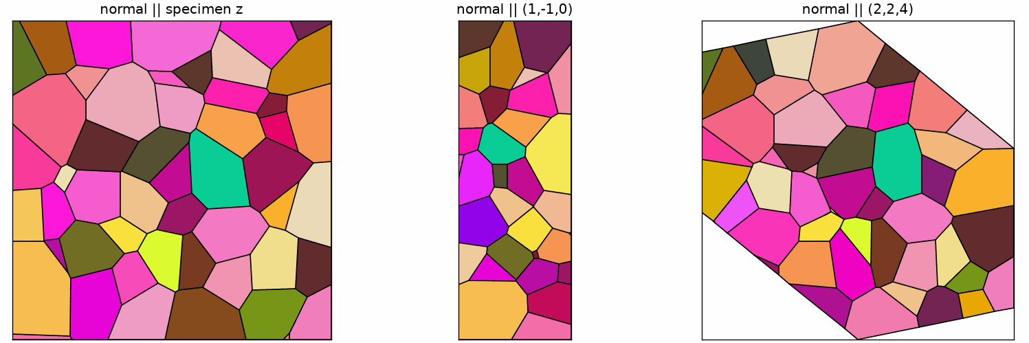
The three panels show differently oriented planes. Their unequal outlines show how the same cuboid and its grains are sampled by horizontal and oblique sections. grains.slice cuts the loaded collection itself, with no external file.

Relate a section to its parent grains

intersected selects the full polyhedra crossed by a plane. Overlaying those grains on the horizontal section connects each planar polygon to the three-dimensional material that produced it.

inPlane = grains.intersected(N[0], A)

plot(grains001, grains001.meanOrientation, micronbar='off')
hold(True)
plot(grains[inPlane], grains[inPlane].meanOrientation, faceAlpha=0.55, edgeAlpha=0.1)
hold(False)
setCamera(how2plot)

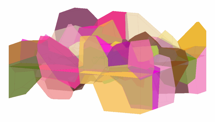
The opaque polygons are the section itself. The translucent polyhedra extend to both sides of the plane and are the corresponding parent grains.

Function reference

References

• R. Quey, P. R. Dawson and F. Barbe, Large-scale 3D random polycrystals for the finite element method: Generation, meshing and remeshing, Computer Methods in Applied Mechanics and Engineering 200 (2011), 1729-1745, presents the generation and meshing methods implemented in Neper.

Next

Continue with Properties of Three-Dimensional Grains to measure the faces, surface area, volume, and shape of the generated collection.

Technical details

neper = neper.init() binds the one interface to the name MATLAB’s static class uses, so that the assignments read as MATLAB’s. The orientations of the simulated grains are sampled at random, so the pictures differ from MATLAB’s in their colours. MATLAB’s neper.getSlice, a section written by Neper to a file, is left out: grains.slice cuts the loaded grains directly.

@article{bachmann2010mtex,
  author  = {F. Bachmann and R. Hielscher and H. Schaeben},
  title   = {Texture Analysis with MTEX - Free and Open Source Software Toolbox},
  journal = {Solid State Phenomena},
  volume  = {160},
  pages   = {63-68},
  year    = {2010},
  doi     = {10.4028/www.scientific.net/SSP.160.63},
  url     = {https://doi.org/10.4028/www.scientific.net/SSP.160.63}
}