Three-Dimensional Grains

In EBSD grain segmentation, a grain is a phase-homogeneous, spatially connected region of pixels produced by segmentation. In three dimensions, MTEX represents its counterpart by the faces of a closed polyhedron and stores a collection as a grain3d object. The faces provide the geometry; phase and mean orientation describe the material inside each polyhedron.

This page follows one collection from import through selection, sectioning, and inspection of its boundary normals. The following pages explain the Neper workflow, geometric properties, and operations on three-dimensional grains in detail.

import numpy as np

from mtex import *

plottingConvention.default('y↑→x')
how2plot = plottingConvention.default3D

Import a DREAM.3D surface mesh

grain3d.load reads a DREAM.3D triangle mesh into a grain3d collection. The voxel data of the same file is read by EBSD3.load and segmented by calcGrains, see Grain Reconstruction.

fname = mtexdatafile('SmallIN100')
grains = grain3d.load(fname)
print(grains)

grain3d (y↑→x)
  Phase  Grains              Mineral  Color         Symmetry  Crystal reference frame
  1      794 (volume 15625)  unknown  LightSkyBlue  432       unknown
  boundary faces: 757564

Read the imported microstructure

The summary reports the phases, number of grains, total volume and boundary faces. Plotting the mean orientation assigns one orientation colour to each polyhedron; it does not display pointwise orientation variation.

plot(grains, grains.meanOrientation, edgeAlpha=0.1, micronbar='off')
setCamera(how2plot)

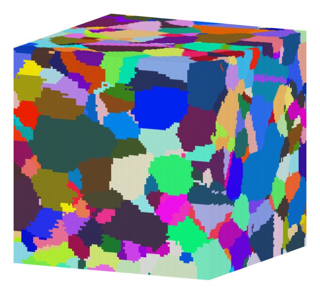
The colour changes sharply at grain contacts. Faint triangle edges reveal the surface mesh while keeping the grain shapes and colours readable. Use edgeAlpha between 0.1 and 0.2 for this balance.

The figure links to an interactive view of the same scene: drag to rotate it, scroll to zoom.

Why face winding matters

A face normal is perpendicular to one boundary face. Its sign follows from the order of the face vertices, called the face winding. DREAM.3D stores faces with arbitrary winding, so the stored normal may point into or out of a grain.

By default, the importer calls orientFaces. MTEX then uses I_GF to record which direction is outward for each grain. This makes signed volumes and boundary.grainId directly usable. Request the raw DREAM.3D winding only when that order is itself needed.

grainsRaw = grain3d.load(fname, orientFaces=False)

The first value below counts negative raw volumes; the second checks the oriented import. Negative values diagnose inconsistent orientation of the enclosing faces; they are not negative amounts of material.

print([np.count_nonzero(grainsRaw.volume < 0), np.count_nonzero(grains.volume < 0)])

[419, 0]

Select a grain

A collection can be indexed by any logical condition. The following code finds the array position of the largest grain and then plots that grain. Grain ids and array positions can differ after subsetting, so use an id query when the persistent identity matters.

id = int(np.argmax(grains.volume))
print(id)

plot(grains[id], edgeAlpha=0.2, micronbar='off')
setCamera(how2plot)

622

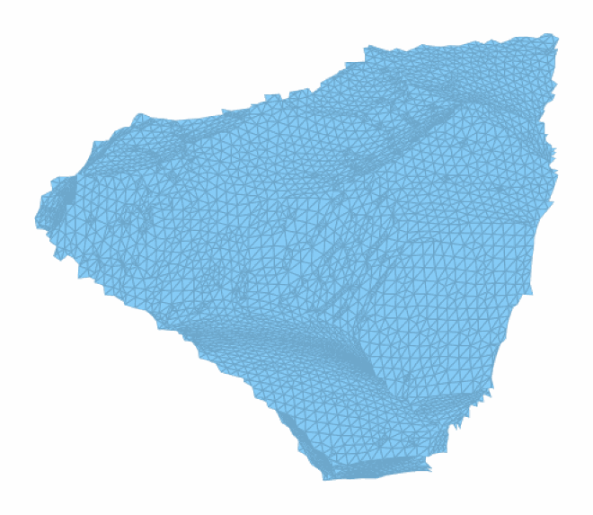
The translucent edges expose the triangular boundary mesh of the selected polyhedron. The result is one three-dimensional grain, not a planar section.

Cut a planar section

A plane3d is defined by a normal direction and a point in the plane. slice intersects that plane with every grain and returns the resulting polygons as a grain2d collection, comparable to what can be reconstructed from a two-dimensional EBSD map.

plane = plane3d(vector3d(1, 1, 1), vector3d(-20, 20, -15))
grains2 = grains.slice(plane)
print(grains2)

plot(grains2, grains2.meanOrientation, micronbar='off')
setCamera(how2plot)

grain2d (y↑→x)
  size: 188
  Phase  Grains            Mineral  Color         Symmetry  Crystal reference frame
  1      188 (188 pixels)  unknown  LightSkyBlue  432       unknown
  boundary segments: 7177, inner: 0, triple points: 271
  properties       : Id3d

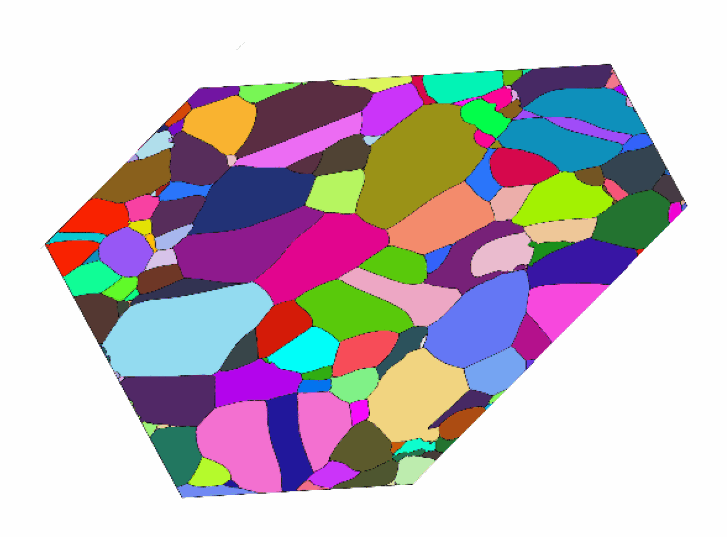
The plot contains only grains crossed by the plane. Each polygon inherits the mean orientation of its parent three-dimensional grain.

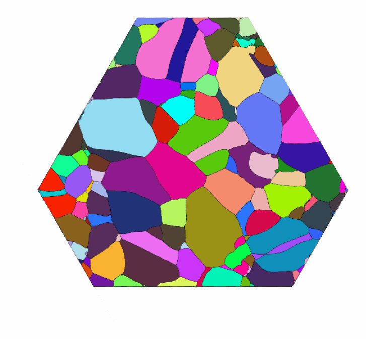
For a face-on view, use a plotting convention whose out-of-screen direction is the section normal. The east direction fixes the remaining in-plane freedom.

how2plot2 = plottingConvention()
how2plot2.outOfScreen = grains2.N
how2plot2.east = vector3d(1, -1, 0)
setCamera(how2plot2)

Look inside the volume

The outer surface hides the neighbourhood of an interior grain. Selecting a few grains exposes the shapes that matter for local constraint and load transfer. The boundary stores persistent grain ids, so selection remains valid even when the collection has been sorted or reduced.

grain = grains[id]
gB = grain.boundary
neighbourIds = np.setdiff1d(np.unique(gB.grainId), np.r_[0, grain.id])
neighbours = grains['id', neighbourIds]

plot(neighbours, neighbours.meanOrientation, faceAlpha=0.2, edgeAlpha=0.1, micronbar='off')
hold(True)
plot(grain, faceColor=[0.85, 0.25, 0.15], edgeAlpha=0.1)
hold(False)
setCamera(how2plot)

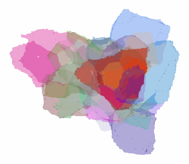
The opaque grain and its translucent neighbours share actual boundary faces. Proximity of their centroids alone would not establish that they touch. Boundary Network measures those contacts and the junctions between them.

Plot outward normals for one grain

A shared face has only one stored normal, so that normal cannot point outwards from both adjacent grains. The corresponding row of I_GF contains the sign needed for the selected grain. Multiplying by that sign produces outward directions.

# select by array position; the boundary keeps the persistent grain ids
id = 2
dir = grains[id].I_GF[0, :].toarray().reshape(-1) * grains[id].boundary.N

plot(grains[id], edgeAlpha=0.2, micronbar='off')
hold(True)
quiver(grains[id].boundary, dir)
hold(False)
setCamera(plottingConvention.default3D)

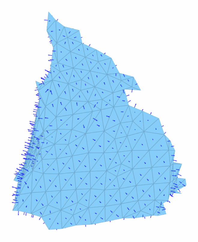
The arrows point away from the selected polyhedron. They represent face normals, not the misorientation between neighbouring grain orientations.

References

• M. A. Groeber and M. A. Jackson, DREAM.3D: A Digital Representation Environment for the Analysis of Microstructure in 3D, Integrating Materials and Manufacturing Innovation 3 (2014), 56-72, describes the data environment and surface-mesh representation used by the importer.

Next

Continue with Grain Reconstruction to build these surfaces from voxel measurements. Neper Interface creates a synthetic comparison, while Properties turns the geometry into size and shape distributions.

Technical details

Positions count from 0: MATLAB’s grain id = 3 is grains[2] here, and the largest grain’s position is one less than MATLAB prints. slice(grains, plane) is the method grains.slice(plane), since slice is a Python builtin. MATLAB’s axis off and empty labels after setCamera have nothing to act on in a 3D scene.

@article{bachmann2010mtex,
  author  = {F. Bachmann and R. Hielscher and H. Schaeben},
  title   = {Texture Analysis with MTEX - Free and Open Source Software Toolbox},
  journal = {Solid State Phenomena},
  volume  = {160},
  pages   = {63-68},
  year    = {2010},
  doi     = {10.4028/www.scientific.net/SSP.160.63},
  url     = {https://doi.org/10.4028/www.scientific.net/SSP.160.63}
}