Grain Reconstruction from Voxel Data

A three-dimensional EBSD measurement arrives as voxels, whether it comes from serial sectioning or from a diffraction technique that probes the volume. Each voxel carries a position, a phase and an orientation. A grain is a phase-homogeneous, spatially connected region of such voxels. This page asks how the segmentation criterion changes the grains we measure. Unlike the simulated multiphase volume in the overview, this example uses the DREAM.3D IN100 data so that one phase can be coloured by orientation.

import matplotlib.pyplot as plt
import numpy as np

from mtex import *

plottingConvention.default('y↑→x')
how2plot = plottingConvention.default3D

Load the voxel data

EBSD3.load reads the cell data of a DREAM.3D file into an EBSD3 on a voxel lattice, the voxel counterpart of a square grid EBSD map. The voxels form a three-dimensional array, so ebsd[i, j, k] addresses one of them. Every further scalar array of the file becomes a property.

fname = mtexdatafile('SmallIN100')
ebsdImported = EBSD3.load(fname)
ebsd = ebsdImported.copy()
print(ebsd)

EBSD3 (y↑→x)
  size: 100 × 100 × 100 grid
  Phase  Orientations    Mineral  Color         Symmetry  Crystal reference frame
  1      1000000 (100%)  unknown  LightSkyBlue  432       unknown
  properties: ConfidenceIndex, FeatureReferenceMisorientations, Fit, GBManhattanDistances, ImageQuality, KernelAverageMisorientations, ParentIds, QPManhattanDistances, SEMSignal, TJManhattanDistances, grainId
  scan unit : um
  X × Y × Z : [-37 → -12.25] × [10.25 → 35] × [-29.25 → -4.5]
  voxel     : 0.25 × 0.25 × 0.25

Reconstruct the grains

calcGrains works as its two-dimensional counterpart: two neighbouring voxels belong to the same grain when their misorientation angle stays below the threshold. Voxels are 6-connected. The boundary between two grains consists of the voxel faces they share, each stored as two triangles, so every grain is a closed surface.

grains = calcGrains(ebsd, angle=5 * degree)
print(grains)

grain3d (y↑→x)
  Phase  Grains              Mineral  Color         Symmetry  Crystal reference frame
  1      812 (volume 15625)  unknown  LightSkyBlue  432       unknown
  boundary faces: 757562

The summary lists the grains with their volume. The voxel data now carries a grainId per voxel. Plotting the mean orientation colours every face on the outside of the volume.

plot(grains, grains.meanOrientation, edgeAlpha=0.1, micronbar='off')
setCamera(how2plot)

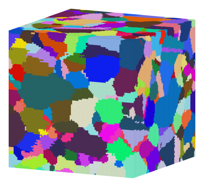
The colour is constant over each grain and changes sharply at the grain boundaries. The staircase texture of the outer faces is the voxel grid itself; the boundary follows the voxel faces exactly.

Volumes

Every grain is a closed surface, so its volume follows from the divergence theorem and equals the number of its voxels times the voxel volume. The volumes of all grains add up to the measured box.

print([grains.volume.sum(), np.prod(ebsd.shape) * ebsd.dx * ebsd.dy * ebsd.dz])

[15625.0, 15625.0]

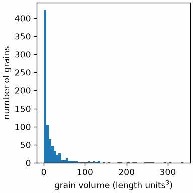
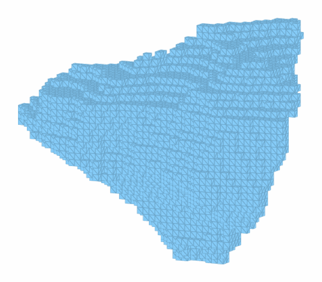
Most grains are small. The largest grain is worth a look on its own.

newMtexFigure()
histogram(grains.volume)
plt.xlabel('grain volume (length units$^3$)')
plt.ylabel('number of grains')

id = int(np.argmax(grains.volume))
plot(grains[id], micronbar='off', edgeAlpha=0.2)
setCamera(how2plot)

Grains stored in the file

DREAM.3D and GrainMapper3D files carry the grain id the vendor software assigned to every voxel, which the importer stores as ebsd.grainId. The flag 'grainId' builds the grains from these ids instead of the orientations, so the stored segmentation becomes a grain3d with the same closed surfaces, volumes and boundary as a reconstruction of our own.

grainsStored = calcGrains(ebsdImported.copy(), 'grainId')
print(grainsStored)

grain3d (y↑→x)
  Phase  Grains              Mineral  Color         Symmetry  Crystal reference frame
  1      813 (volume 15625)  unknown  LightSkyBlue  432       unknown
  boundary faces: 757564

calcGrains replaces ebsd.grainId, so the stored segmentation must be read from a copy of ebsdImported. Grain labels are arbitrary: subtracting the two id arrays would not measure agreement. First compare a physically meaningful quantity, the equivalent-sphere diameter, \(d_V=(6V/\pi)^{1/3}\), for indexed grains in each reconstruction.

gMTEX = grains['indexed']
gStored = grainsStored['indexed']
dMTEX = (6 * gMTEX.volume / np.pi) ** (1 / 3)
dStored = (6 * gStored.volume / np.pi) ** (1 / 3)
diameterEdges = np.linspace(0, max(dMTEX.max(), dStored.max()), 25)

newMtexFigure()
histogram(dMTEX, diameterEdges, label='MTEX, 5 degrees')
hold(True)
histogram(dStored, diameterEdges, label='stored segmentation', alpha=0.7)
hold(False)
plt.legend(loc='best')
plt.xlabel('equivalent-sphere diameter (length units)')
plt.ylabel('number of grains')

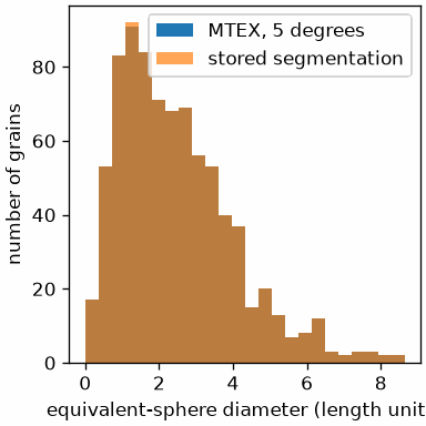
Similar distributions do not establish voxel-by-voxel agreement. They do show whether the two segmentations give similar grain sizes. To locate discrepancies, compare their grainId properties on the same slice.

Small grains

A handful of voxels with a stray orientation form a grain of their own. The option minPixel removes indexed grains below a number of voxels. Their voxels are marked notIndexed and form notIndexed grains, exactly as in two dimensions.

ebsdClean = ebsdImported.copy()
grainsClean = calcGrains(ebsdClean, angle=5 * degree, minPixel=10)
print([len(grains['indexed']), len(grainsClean['indexed'])])

[812, 749]

A cutoff is a choice of minimum resolved volume: ten voxels correspond to the volume below. It can suppress isolated indexing errors, but also remove real small grains. Check the affected regions before interpreting a loss of fine grains as a material feature.

minimumVolume = 10 * ebsd.dx * ebsd.dy * ebsd.dz
print(minimumVolume)
removedFraction = np.count_nonzero(ebsdImported.isIndexed & ~ebsdClean.isIndexed) / np.count_nonzero(ebsdImported.isIndexed)
print(removedFraction)

0.15625
0.000252

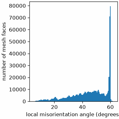
The grain boundary

grains.boundary is a grain3Boundary. Each face records the two voxels it separates, ebsdId, the two grains, grainId, and the misorientation between the two voxels. Faces on the outside of the volume have a zero in the second column of grainId. The misorientation angle across the inner faces shows where the low angle boundaries are.

gB = grains.boundary
isInner = np.all(gB.grainId > 0, axis=1) & np.all(gB.isIndexed, axis=1)
newMtexFigure()
histogram(gB[isInner].misorientation.angle() / degree)
plt.xlabel('local misorientation angle (degrees)')
plt.ylabel('number of mesh faces')

Next

Smoothing removes voxel steps before surface measurements. Properties measures the reconstructed grains, and Operations relates sections to their parent grains. Boundary Network measures internal interfaces. The Three-Dimensional Grains page reads the surface mesh DREAM.3D stored alongside the voxels.

Technical details

calcGrains alters the volume it is given, writing its grain ids and the voxels minPixel removes into it, where MATLAB returns an altered copy as a second output. MATLAB’s ebsd = ebsdImported is therefore ebsdImported.copy() here, and each reconstruction to be compared runs on a copy of its own.

@article{bachmann2010mtex,
  author  = {F. Bachmann and R. Hielscher and H. Schaeben},
  title   = {Texture Analysis with MTEX - Free and Open Source Software Toolbox},
  journal = {Solid State Phenomena},
  volume  = {160},
  pages   = {63-68},
  year    = {2010},
  doi     = {10.4028/www.scientific.net/SSP.160.63},
  url     = {https://doi.org/10.4028/www.scientific.net/SSP.160.63}
}