Volume Data and Slices

An EBSD3 object stores one measurement per voxel: its position, phase, orientation, and whatever properties the file provides. It is the volume counterpart of a two-dimensional EBSD map, and the representation to use while the question still concerns individual measurements rather than whole-grain geometry.

This page imports such a volume, displays it, and cuts planar slices out of it. A slice is an ordinary two-dimensional EBSD map, so everything written for planar data applies to it unchanged. The polyhedral grain3d representation is the subject of Three-Dimensional Grains.

from mtex import *

plottingConvention.default('y↑→x')

Import a volume

EBSD3.load detects the file format automatically. The sample data set is a simulated nine-phase volume written in the Xnovo GrainMapper3D format,

ebsd = EBSD3.load(os.path.join(mtexDataPath(), 'EBSD3', 'SimulatedMultiPhase.h5'))

which mtexdata resolves by name.

ebsd = mtexdata('xnovo')
print(ebsd)

EBSD3 (y↑→x)
  size: 50 × 50 × 50 grid
  Phase  Orientations  Mineral     Color                Symmetry  Crystal reference frame
  0      27950 (22%)   notIndexed
  1      11046 (8.8%)  Silicon     [0.584 0.878 0.969]  m-3m      Silicon
  2      11876 (9.5%)  Diamond     [0.82  0.31  0.467]  m-3m      Diamond
  3      10436 (8.3%)  Magnesium   [1. 0. 0.]           6/mmm     Magnesium
  4      10231 (8.2%)  Rutile      [1. 0. 0.]           4/mmm     Rutile
  5      9060 (7.2%)   Corundum    [0.714 0.839 0.471]  -3m1      Corundum
  6      11521 (9.2%)  Quartz      [0.    0.698 0.875]  -3m1      Quartz
  7      10961 (8.8%)  Pyroxene    [0.929 0.604 0.345]  mmm       Pyroxene
  8      10578 (8.5%)  Hornblende  [0.733 0.467 0.773]  12/m1     Hornblende
  9      11341 (9.1%)  Microcline  [0.969 0.851 0.388]  -1        Microcline
  properties: Completeness, grainId
  scan unit : mm
  X × Y × Z : [-0.245 → 0.245] × [-0.245 → 0.245] × [-0.245 → 0.245]
  voxel     : 0.01 × 0.01 × 0.01

The summary reports a 50 x 50 x 50 grid rather than a list, i.e. the measurements are held on a lattice whose entries are addressed as ebsd[i, j, k]. The three array dimensions carry \(x\), \(y\) and \(z\). Each of the nine phases occupies roughly a twelfth of the voxels and the remaining fifth is not indexed.

The voxel is 10 micron on a side and the volume spans about half a millimetre in each direction.

print([ebsd.dx, ebsd.dy, ebsd.dz])
print(ebsd.extent())

[0.01, 0.01, 0.01]
[-0.245  0.245 -0.245  0.245 -0.245  0.245]

Select voxels

A phase or a condition selects voxels the way it selects the pixels of a map. The result is a list of the selected voxels, shorter than the volume, that still carries the unit cell of the grid it came from.

ebsdQuartz = ebsd['Quartz']
print(ebsdQuartz)

EBSD3 (y↑→x)
  size: 11521
  Phase  Orientations  Mineral  Color                Symmetry  Crystal reference frame
  6      11521 (100%)  Quartz   [0.    0.698 0.875]  -3m1      Quartz
  properties: Completeness, grainId
  scan unit : mm
  X × Y × Z : [-0.235 → 0.245] × [-0.235 → 0.245] × [-0.245 → 0.245]
  voxel     : 0.01 × 0.01 × 0.01

Whatever needs the grid rebuilds it in place: calcGrains, plot and slice put the list back onto its lattice, with the cells nobody occupies not indexed, and gridify does so explicitly. A block of subscripts, ebsd[9:20, 9:20, 9:20], keeps the grid and crops it.

Display the volume

plot shows the volume in three slice planes through its middle, the picture MATLAB’s volume viewer opens with. The figure links to an interactive page of the same scene, and show3d() opens it in a window where it is rotated and zoomed with the mouse:

plot(ebsd)                          # colour by phase
plot(ebsd, ebsd.prop['grainId'])    # colour by a property

plot(ebsd)

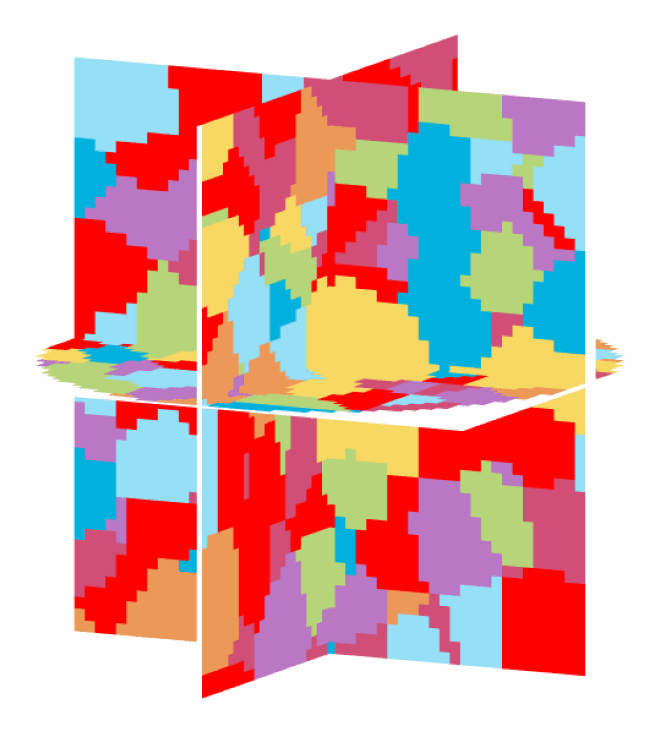
Voxel colours are never interpolated, so a boundary stays where the measurement puts it, and voxels that are not indexed are painted in white. The planes lie at the middle voxel of each axis; plot(ebsd, at=(i, j, k)) puts them elsewhere.

Anything that has to end up in a figure, a publication, or a further calculation goes through a slice.

Cut a slice

slice resamples the volume onto a regular grid inside a plane3d and returns a two-dimensional EBSD map. The plane is given by its normal and one point on it.

ebsdZ = ebsd.slice(plane3d(vector3d.Z, vector3d(0, 0, 0)))
print(ebsdZ)

EBSD (y↑→x)
  size: 52 × 52 grid
  Phase  Orientations  Mineral     Color                Symmetry  Crystal reference frame
  0      763 (28%)     notIndexed
  1      376 (14%)     Silicon     [0.584 0.878 0.969]  m-3m      Silicon
  2      122 (4.5%)    Diamond     [0.82  0.31  0.467]  m-3m      Diamond
  3      179 (6.6%)    Magnesium   [1. 0. 0.]           6/mmm     Magnesium
  4      128 (4.7%)    Rutile      [1. 0. 0.]           4/mmm     Rutile
  5      193 (7.1%)    Corundum    [0.714 0.839 0.471]  -3m1      Corundum
  6      76 (2.8%)     Quartz      [0.    0.698 0.875]  -3m1      Quartz
  7      256 (9.5%)    Pyroxene    [0.929 0.604 0.345]  mmm       Pyroxene
  8      236 (8.7%)    Hornblende  [0.733 0.467 0.773]  12/m1     Hornblende
  9      375 (14%)     Microcline  [0.969 0.851 0.388]  -1        Microcline
  properties    : Completeness, grainId
  scan unit     : mm
  X × Y         : [-0.255 → 0.255] × [-0.255 → 0.255]
  square lattice: spacing 0.01

The result is a gridded map like any imported one, it carries all nine phases, and it plots like one.

plot(ebsdZ)

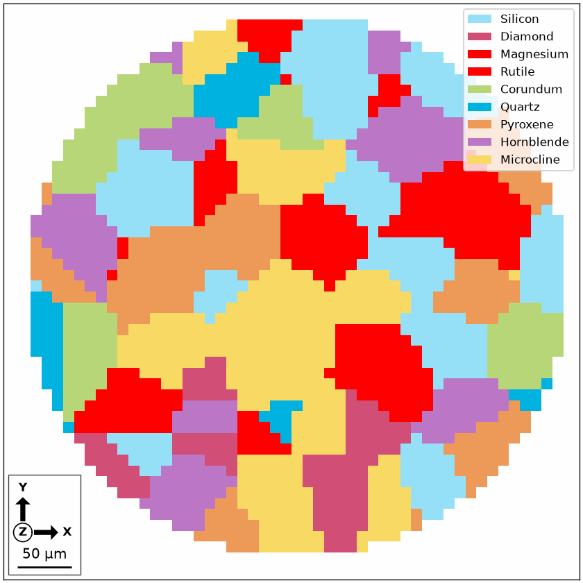
The section is a disc, so the simulated specimen is round in the \(xy\) plane rather than filling its bounding box. The grains are equiaxed and the nine phases are mixed through the section without any layering.

Slices at several depths

Repeating the cut at different heights shows how the microstructure develops through the volume. Each panel is a full EBSD map.

newMtexFigure(layout=[1, 3], figSize='large')

for z in [-0.15, 0, 0.15]:
  plot(ebsd.slice(plane3d(vector3d.Z, vector3d(0, 0, z))), micronbar='off')
  mtexTitle(f'z = {z:g} mm')
  if z < 0.15:
    nextAxis()

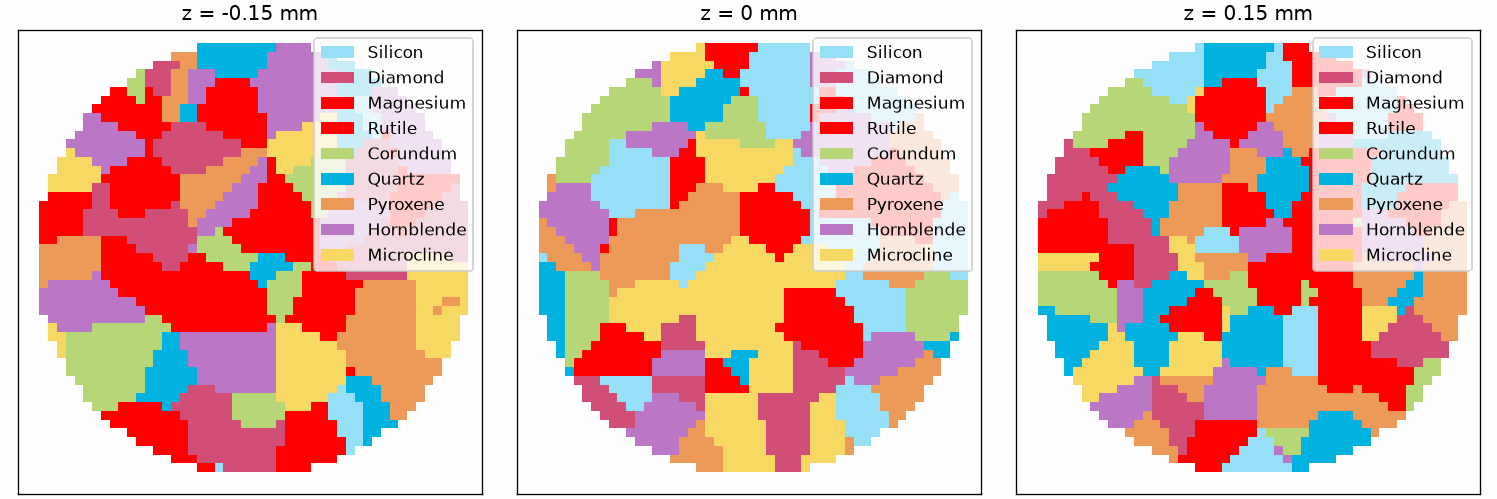
The three discs have the same diameter, so the specimen is a cylinder standing along \(z\). The grain pattern is different in each panel because every section meets a different set of grains.

An arbitrary plane

The normal is unrestricted. The measurements of a section keep their position in the specimen, and a map is drawn in the coordinates of the plane it lies in, so a section that does not lie in the \(xy\) plane is drawn face on without moving any data.

newMtexFigure(layout=[1, 2], figSize='large')

plot(ebsd.slice(plane3d(vector3d.X, vector3d(0, 0, 0))), micronbar='off')
mtexTitle('normal || x')
nextAxis()
plot(ebsd.slice(plane3d(vector3d(1, 1, 1), vector3d(0, 0, 0))), micronbar='off')
mtexTitle('normal || (1,1,1)')

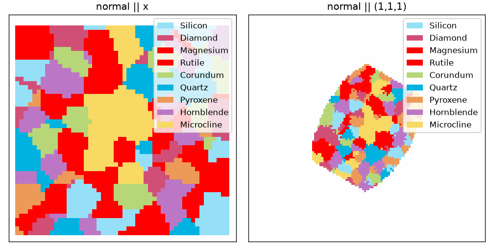
The section normal to \(x\) is rectangular and shows the full height of the cylinder. The oblique section is the larger of the two because that plane crosses more of the specimen; its grid is regular within the plane, not in the specimen axes.

Several sections at once

A section keeps the position its measurements have in the specimen, so drawing more than one into the same axes assembles them where they belong. Three orthogonal cuts seen from an angle give the picture the volume viewer shows, in a figure that can be published.

plot(ebsd.slice(plane3d(vector3d.Z, vector3d(0, 0, 0))), micronbar='off')
hold(True)
plot(ebsd.slice(plane3d(vector3d.X, vector3d(0, 0, 0))), micronbar='off')
plot(ebsd.slice(plane3d(vector3d.Y, vector3d(0, 0, 0))), micronbar='off')
hold(False)

setCamera(plottingConvention.default3D)

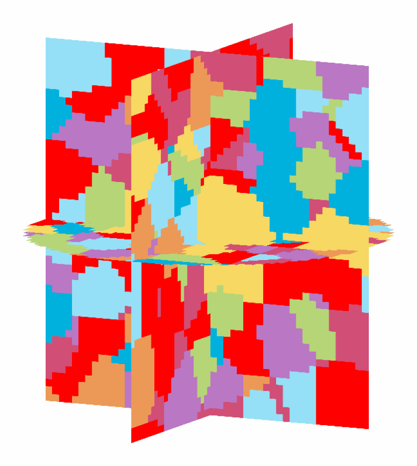
The convention a single section carries decides how that section alone is seen. Once several are combined there is one camera for all of them, and plottingConvention.default3D is the oblique view this chapter uses. The three planes meet at the centre of the specimen, so a grain crossed by two of them appears in both.

Colour a slice

A slice carries the orientations, phases and properties of the voxels it passes through, so it is coloured by exactly the same commands as an imported map. Orientation colouring needs a single phase at a time, which for a multi-phase section means one call per phase.

for p in ebsdZ.indexedPhaseId:
  ebsdP = ebsdZ[ebsdZ.CSList[p].mineral]
  plot(ebsdP, ebsdP.orientations, micronbar='off')
  hold(True)
hold(False)

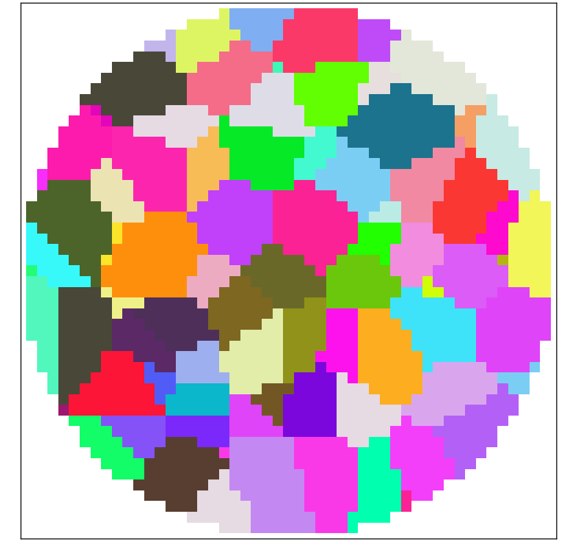
Each phase is coloured by its own inverse pole figure key, so colours are comparable within a phase but not between phases.

Separate orientation from measurement quality

A dark or abruptly changing orientation colour does not by itself indicate a poor measurement. Compare a stored quality field with orientation on the same plane. Completeness is supplied by this Xnovo file; other importers may provide different quality measures.

newMtexFigure(layout=[1, 2], figSize='large')
plot(ebsdZ, ebsdZ.prop['Completeness'], micronbar='off')
mtexTitle('Completeness')
mtexColorbar()
nextAxis()
quartz = ebsdZ['Quartz']
ipfKey = ipfColorKey(quartz.CS)
ipfKey.inversePoleFigureDirection = vector3d.Z
plot(quartz, ipfKey.orientation2color(quartz.orientations), micronbar='off')
mtexTitle('Quartz: IPF along specimen z')

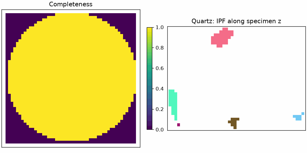
The IPF reference is a specimen direction. It stays along \(z\) even when the cutting plane or camera changes. Reuse the same key when comparing orientations on several sections. Interpret completeness using the acquisition method; this simulated example does not establish a cutoff for experimental data.

A slice is an ordinary EBSD map

Nothing distinguishes the result of slice from an imported map, so the planar toolchain applies to it directly. Here the section is segmented into grains and the boundaries drawn over the phase map.

grains = calcGrains(ebsdZ)

plot(ebsdZ, micronbar='off')
hold(True)
plot(grains.boundary, lineWidth=2)
hold(False)

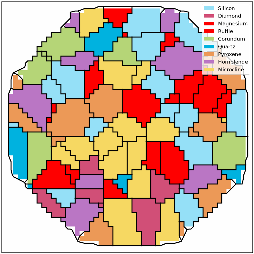
These are grains reconstructed independently in two dimensions. A grain connected outside this plane can appear as separate regions here, so this segmentation need not match a slice of the three-dimensional grains. This data set also ships the segmentation of the full volume as the voxel property grainId, which the slice carries along.

Reconstructing grains in the volume as closed polyhedra is described in Three-Dimensional Grains.

Function reference

References

• F. Bachmann, R. Hielscher, and H. Schaeben, Grain Detection from 2d and 3d EBSD Data - Specification of the MTEX Algorithm, Ultramicroscopy 111 (2011), 1720-1733, specifies the segmentation that calcGrains applies to the section.

Next

Continue with Three-Dimensional Grains to turn a volume into polyhedra and to work with their faces and normals.

Technical details

MATLAB’s plot(ebsd) opens its interactive volume viewer, which a page cannot hold; here it draws the three middle slices as a figure with an interactive page. slice(ebsd, plane) is the method ebsd.slice(plane), since slice is a Python builtin, and a section is drawn face on in the coordinates of its plane rather than through a plotting convention of its own.

@article{bachmann2010mtex,
  author  = {F. Bachmann and R. Hielscher and H. Schaeben},
  title   = {Texture Analysis with MTEX - Free and Open Source Software Toolbox},
  journal = {Solid State Phenomena},
  volume  = {160},
  pages   = {63-68},
  year    = {2010},
  doi     = {10.4028/www.scientific.net/SSP.160.63},
  url     = {https://doi.org/10.4028/www.scientific.net/SSP.160.63}
}