SO3Fun.plotPDF

pole figures, one per crystal direction: of an ODF, of a list of orientations or of a measured PoleFigure; MATLAB’s plotPDF

Syntax

plotPF(odf, h)

plotPF(odf, h, superposition=[0.5, 0.5])

plotPF(ori, h)

plotPF(ori, ori.angle(), h)

plotPF(ori, h, contourf=True, antipodal=True)

plotPF(ori, h, points=50)

plotPF(ori, h, all=True)

plotPF(f, Miller(1, 0, 0, f.CS))

plotPF(pf)

Description

A pole figure shows where the crystal direction h, with every equivalent of it, points in the specimen. For an ODF it is the density of these poles, the Radon transform odf.radon(h), drawn with the keywords of a spherical function: contourf, contour, pcolor, colorRange (‘equal’ for one range over all pole figures, each its own by default), resolution, antipodal (both hemispheres superposed), complete, upper and lower. A positional ‘3d’ draws it on the sphere in space.

For a list of orientations every orientation is applied to every equivalent of h and the poles are drawn as markers on the specimen sector, coloured by a value or an RGB colour per orientation when one is given; contourf=True or another filled style draws their density. A large list is thinned to a random selection, about 10000 markers by default. A fibre is drawn as the dots of 1000 orientations along it. Into held pole figures, or with add2all=True, the poles of the directions already shown are added.

A measured PoleFigure draws its intensities as markers, or, with a filled style, the function its harmonic expansion gives.

Input

Keywords

Example

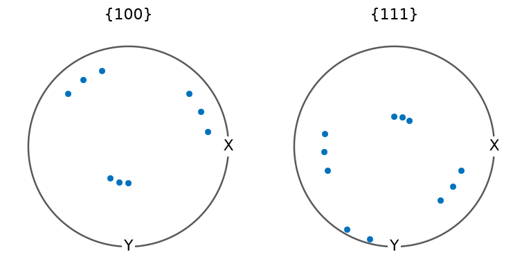
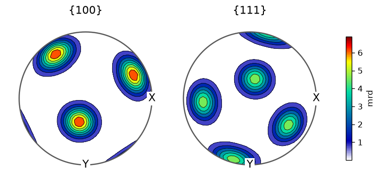
Compare poles of three explicit orientations with the pole density of a model ODF. Each plot contains the cubic {100} and {111} families; antipodal=True identifies opposite poles.

import numpy as np
import matplotlib.pyplot as plt
from mtex import crystalFrame, orientation, Miller, degree, plotPF, unimodalODF, mtexColorbar

cs = crystalFrame('m-3m')
h = [Miller(1, 0, 0, cs), Miller(1, 1, 1, cs)]
ori = orientation.byEuler(np.array([0, 15, 30])*degree, 30*degree, 45*degree, cs)
plotPF(ori, h, all=True, antipodal=True, markerSize=5)
centre = orientation.byEuler(15*degree, 30*degree, 45*degree, cs)
odf = unimodalODF(centre, halfwidth=15*degree)
plotPF(odf, h, antipodal=True, contourf=True, resolution=5*degree, colorRange='equal')
mtexColorbar(title='mrd')
plt.show()

The first figure shows discrete poles. The second shows a continuous density in multiples of a random distribution; it is the projection of the model ODF, not a fit to those three orientations.

See also

plotIPF, SO3Fun.radon, PoleFigure, calcPoleFigure, annotate, ODFPoleFigure, OrientationPoleFigure, PoleFigurePlot

Used on

CrystalReferenceSystem, OrientationFibre, OrientationGrid, OrientationImport, OrientationPoleFigure, OrientationStandard, OrientationSymmetry, SpecimenSymmetry, EBSD2ODF, EBSDOrientationAnalysis, EBSDOrientationPlots, EBSDReferenceFrame

MATLAB’s SO3Fun.plotPDF

@article{bachmann2010mtex,
  author  = {F. Bachmann and R. Hielscher and H. Schaeben},
  title   = {Texture Analysis with MTEX - Free and Open Source Software Toolbox},
  journal = {Solid State Phenomena},
  volume  = {160},
  pages   = {63-68},
  year    = {2010},
  doi     = {10.4028/www.scientific.net/SSP.160.63},
  url     = {https://doi.org/10.4028/www.scientific.net/SSP.160.63}
}