ODF Import

Importing an orientation distribution function (ODF) means creating an MTEX function from a file. The file may preserve an MTEX function exactly, or it may contain only a finite table from which a function must be reconstructed. Those are different operations even when both files contain Euler angles and a fourth numeric column.

This page assumes the density and mrd normalization introduced in ODF Theory. It also assumes the orientation map, Euler-angle conventions, and reference frames introduced in Defining Orientations. Importing Crystal Orientations details the generic text importer and its current limitations.

MTEX supports the following common cases:

• a pickle file with an MTEX ODF object – lossless and binary;
• an MTEX ASCII file containing its components – lossless for the supported component representations;
• a VPSC file containing weighted discrete orientations;
• a generic text table containing Euler angles and values or weights.

The MTEX ASCII description is intended to preserve supported components. In the current source tree, however, SO3Fun.load has loaders only for generic and VPSC ODF files. There is no matching reader of the MTEX component file. Use pickle when an exact round trip matters.

The simplest interactive route in MATLAB is the import wizard, which is not ported. It browses a folder and shows what each file contains. It can either create a variable or write an import script. The following example has the same form as that script.

from mtex import *

# State how specimen x and y are drawn. This changes only the screen layout;
# it does not rotate the imported orientations or change their reference frame.
plottingConvention.default('y↑→x')

# define the crystal and specimen symmetries named in the file header
cs = crystalFrame('m-3m')
ss = specimenFrame('1')

# the file name
fname = mtexdatafile('odf')

# load the data as tabulated function values
odfInterp = SO3Fun.load(fname, 'Bunge', 'interp', CS=cs, SS=ss, columnNames=['Euler 1', 'Euler 2', 'Euler 3', 'weights'])

# plot the imported function
plot(odfInterp, sections=6, verbose=False)

  Interpolating the ODF. This might take some time...

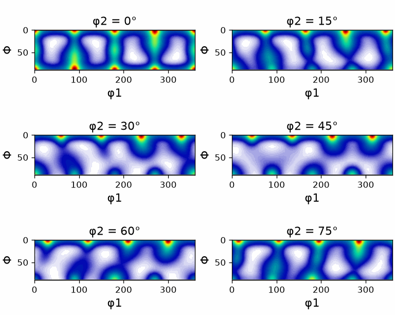
The panels are sections through one three-dimensional function, not six separate pole figures. They reveal localized high-density regions in the imported texture. They do not reveal whether the fourth column was meant as function values or component masses. Either interpretation can produce a plausible texture plot.

The file header calls its fourth column value. The logical name 'weights' above merely tells the generic loader which column to use. The explicit 'interp' flag records that the file contains function values instead of leaving that decision to the importer’s heuristic.

What the Weights Mean

A generic ASCII table fixes orientations at finitely many points. It says nothing about the function between them. Its fourth column is also ambiguous. It may either

1. give the value of the ODF at that orientation, or
2. give the volume of a bell-shaped component centred there.

A heading such as weight does not settle the question. The exporting program’s documentation must say which quantity was written. MTEX therefore needs an interpretation, and that interpretation changes the resulting ODF.

An ODF value is a density in multiples of a random distribution (mrd), not the volume fraction at one exact orientation. Volume fractions are integrals over regions of orientation space. See ODF Characteristics.

Interpolation

The flag 'interp' used above reads the fourth column as sampled function values. MTEX then seeks a function that reproduces the tabulated values at the imported orientations.

print(f'interpolation             : mean {mean(odfInterp):.3f}, texture index {norm(odfInterp) ** 2:.3f}, maximum {max(odfInterp)[0]:.2f} mrd')

interpolation             : mean 1.000, texture index 1.205, maximum 3.50 mrd

The mean checks normalization. The texture index and maximum describe concentration, not volume fractions. They are useful here because the same rows will next be given the other interpretation.

For this file, MATLAB’s default least-squares solver reports that it reached its iteration limit. The returned function is normalized, but that warning means convergence has not been established. Do not silence it. The options tol and maxIter control termination, and the fitted values must be checked against the source table when interpolation accuracy matters.

Density Estimation

The flag 'density' reads the fourth column as component masses. This is kernel density estimation: MTEX centres a bell-shaped kernel at every imported orientation and scales it by the corresponding mass.

The file does not contain the kernel halfwidth. It is a genuine free parameter. A narrow kernel leaves the individual components standing, whereas a wide kernel smears the texture out. The halfwidth must therefore come from knowledge of how the data were produced.

halfwidths = [5, 10, 20]
odfDensity = []
for hw in halfwidths:
  odfDensity.append(SO3Fun.load(fname, 'Bunge', 'density', CS=cs, SS=ss, halfwidth=hw * degree,
                                columnNames=['Euler 1', 'Euler 2', 'Euler 3', 'weights']))
  print(f'density, halfwidth {hw:2d} degrees: mean {mean(odfDensity[-1]):.3f}, texture index {norm(odfDensity[-1]) ** 2:.3f}, '
        f'maximum {max(odfDensity[-1])[0]:.2f} mrd')

density, halfwidth  5 degrees: mean 1.000, texture index 1.177, maximum 3.11 mrd
density, halfwidth 10 degrees: mean 1.000, texture index 1.117, maximum 2.35 mrd
density, halfwidth 20 degrees: mean 1.000, texture index 1.030, maximum 1.55 mrd

The printed means remain one, while the texture index and maximum fall as the halfwidth increases. Smoothing redistributes the same normalized mass over a larger part of orientation space.

The four {100} pole-density plots below compare the explicit interpolation with the three density estimates on one colour range. They all came from the same table. Notice how changing only the interpretation and halfwidth changes both the sharpness and peak height.

h = Miller(1, 0, 0, cs)
odfVariants = [odfInterp] + odfDensity
variantName = ['tabulated values', 'density, 5 degrees', 'density, 10 degrees', 'density, 20 degrees']

mtexFig = newMtexFigure(layout=[1, 4], figSize='large')
for i in range(len(odfVariants)):
  plotPF(odfVariants[i], h, antipodal=True, contourf=True, title=False)
  mtexTitle(variantName[i])
  if i < len(odfVariants) - 1:
    nextAxis()
setColorRange('equal')
mtexColorbar(title='mrd')

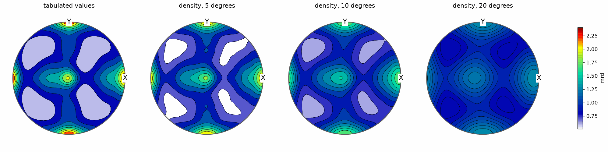
Optimal Kernel Selection discusses halfwidth choice when the file contains a discrete sample of orientations. It cannot recover a halfwidth that an exporting program used before writing sampled ODF values.

When No Interpretation Is Specified

Without either flag, the generic importer uses a heuristic. Varying weights are interpreted as tabulated values, whereas equal weights are treated as a discrete sample for density estimation. This is convenient, but it cannot recover the meaning intended by the program that wrote the file. The varying values in this example would select interpolation, but a reusable script should still specify 'interp' or 'density' explicitly.

Validate the Import

Successful parsing is not validation. Check all of the following against the exporting program and a known feature of the specimen:

• the Euler-angle convention and whether the stored map is active or passive;
• degrees or radians;
• crystal symmetry and the alignment of the crystal frame with the lattice;
• specimen symmetry and the physical directions of the specimen frame;
• the meaning of the fourth column and, for density estimation, the halfwidth.

The generic importer treats an Euler table as degrees only when at least one angle exceeds 15. A degree-valued file confined to smaller angles is silently read as radians. The radians flag cannot force such a file to be read as degrees, so inspect the original scale rather than trusting the plot.

A reference frame is the coordinate system in which the data are expressed. It is distinct from the symmetry attached to that frame. The point group alone does not specify an alignment such as X || a*, Z || c. See The Crystal Reference System and Specimen Symmetry before assigning either one.

The mean ODF should normally be one. Pole figures, sections, and important peak locations should agree with the source. A plausible plot is not enough to distinguish a swapped axis from a genuinely different texture. When possible, map one known crystal direction into a known specimen direction. This breaks ambiguities that visual similarity can hide.

References

• H.-J. Bunge, Texture Analysis in Materials Science: Mathematical Methods, Butterworths, English ed., 1982, establishes ODF normalization and the Bunge Euler convention.
• H. Schaeben, Towards statistics of crystal orientations in quantitative texture analysis, Journal of Applied Crystallography 26 (1993), 112–121, develops kernel orientation-density estimation and its smoothing parameter.
• M. M. Schmitt et al., Texture measurements on quartz single crystals to validate coordinate systems for neutron time-of-flight texture analysis, Journal of Applied Crystallography 56 (2023), 1764–1775, demonstrates why software and specimen frames must be checked with a known asymmetric feature.
• R. A. Lebensohn and C. N. Tomé, A self-consistent anisotropic approach for the simulation of plastic deformation and texture development of polycrystals, Acta Metallurgica et Materialia 41 (1993), 2611–2624, introduces the VPSC formulation behind the weighted-orientation format.

Next

ODF Export explains what information each output format preserves. Visualizing ODFs develops the section and pole-density views used to validate a result. Continue with ODF Characteristics when the imported function should be summarized by peak value, texture index, entropy, or volume fraction. VPSC deformation histories are handled in Import from VPSC.

Technical Details

The table is the sample file mtexdatafile('odf'), fetched on first use, where MATLAB names it under its data folder. The interpolation fits a harmonic series through the values by a regularised least squares, SO3Fun.interpolate, so it returns an SO3FunHarmonic where MATLAB fits a radial function and warns about its iteration limit; its numbers differ accordingly. The import wizard is not ported.

@article{bachmann2010mtex,
  author  = {F. Bachmann and R. Hielscher and H. Schaeben},
  title   = {Texture Analysis with MTEX - Free and Open Source Software Toolbox},
  journal = {Solid State Phenomena},
  volume  = {160},
  pages   = {63-68},
  year    = {2010},
  doi     = {10.4028/www.scientific.net/SSP.160.63},
  url     = {https://doi.org/10.4028/www.scientific.net/SSP.160.63}
}