Import from VPSC

A VPSC simulation can record how a polycrystal’s orientations and slip activity change with strain. This page imports both histories and shows how to compare their deformation steps in MTEX.

VPSC is a crystal-plasticity code originally written by Ricardo Lebensohn and Carlos Tomé at Los Alamos National Laboratory. The original code can be requested from lebenso@lanl.gov.

import os

import matplotlib.pyplot as plt
import numpy as np

from mtex import *

Import the texture history

A VPSC run usually writes TEX_PH1.OUT for phase 1. The file contains one block of weighted orientations for each recorded strain level. It does not contain crystal symmetry, so supply that information first.

cs = crystalFrame('222', [4.762, 10.225, 5.994], mineral='olivine')

SO3Fun.load reads each block and estimates an orientation distribution function (ODF) from its weighted orientations. The halfwidth is the smoothing width of that estimate; it is not a parameter read from VPSC.

mtexdatafile('vpsc')
path2file = os.path.join(mtexDataPath(), 'VPSC')
odf = SO3Fun.load(os.path.join(path2file, 'TEX_PH1.OUT'), halfwidth=10 * degree, CS=cs)

A file with several blocks returns a list with one ODF per block. This sample contains nine ODFs. Its first eight steps run from strain 0.25 to 2.00, and the final block is another result at strain 2.00.

strain = np.array([f.opt.strain for f in odf])
strain

array([0.25, 0.5 , 0.75, 1.  , 1.25, 1.5 , 1.75, 2.  , 2.  ])

Inspect one deformation step

Index the list to select one ODF. A sigma-section plot exposes the three-dimensional orientation density as a sequence of two-dimensional sections.

plotSection(odf[1], 'sigma', figSize='normal')

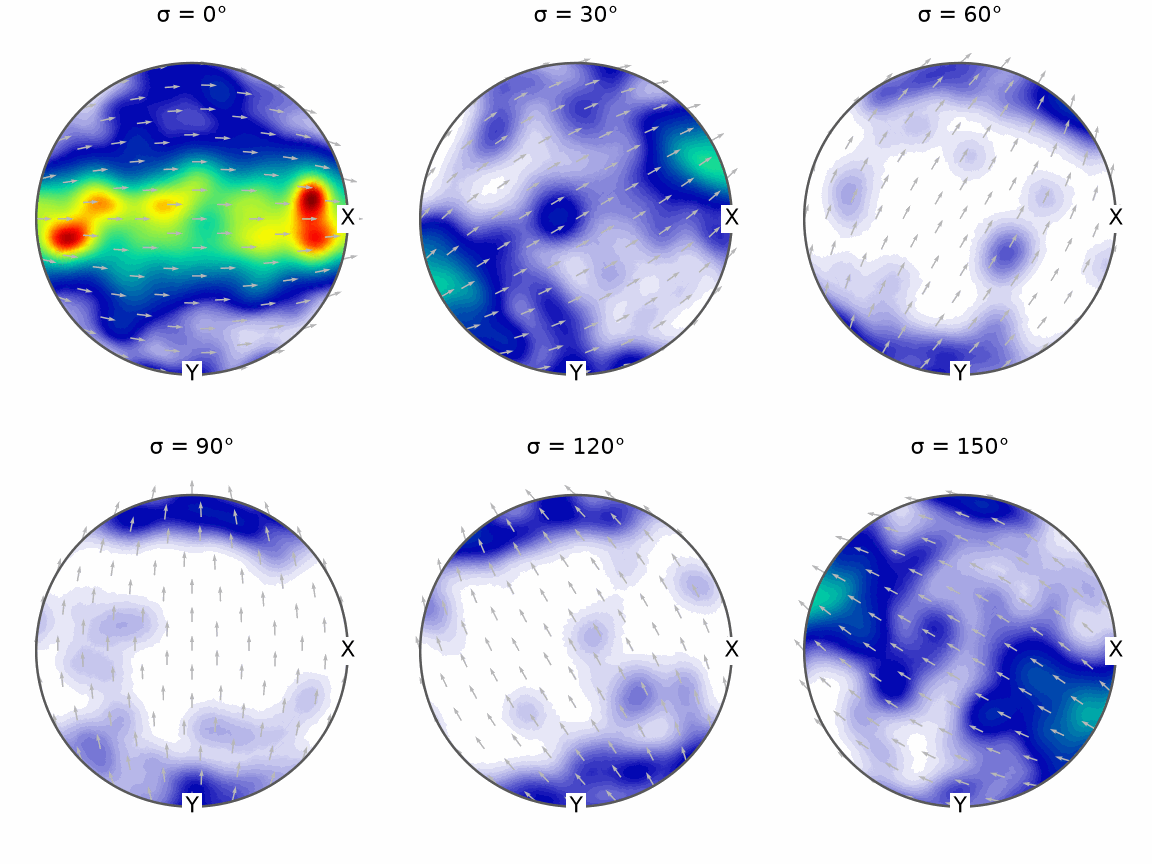
The section maxima identify the preferred orientations at strain 0.50. Their unequal intensities show that this simulated texture is already far from a uniform orientation distribution.

VPSC header values and the original orientation table remain available in opt. The fields below contain the strain, the phase-ellipsoid axes and angles, the 1000 imported orientations, and the three extra numeric columns from this file.

odf[0].opt

namespace(strain=0.25, strainEllipsoid=array([1.123, 1.127, 0.75 ]), strainEllipsoidAngles=array([-180.,   90., -180.]), orientations=orientation (olivine → y↓→x)
  size: 1000
  Bunge Euler angles in degree
  phi1   Phi  phi2
  49.9  90.9  17.4
   111  77.7   277
  39.3  65.3  94.3
   279  37.6  74.3
  12.4   155   171
     ⋮     ⋮     ⋮
   210   103   255
   275  94.6   292
   260  56.8   101
   123    85   256
   241  73.8    95, data=array([[0.3148, 2.787 , 0.8773],
       [0.374 , 4.4999, 1.6829],
       [0.3929, 4.2229, 1.6593],
       ...,
       [0.2259, 4.0012, 0.904 ],
       [0.3761, 4.7342, 1.7804],
       [0.3486, 4.6434, 1.6187]]))

File conventions and input weight files

The same command reads weight files with the .wts extension that are handed to VPSC. It also reads files written by export(ori, fname, 'VPSC'). Those files carry neither strain nor a phase ellipsoid, so the corresponding odf.opt entries are NaN.

The fourth header line names the Euler-angle convention. VPSC uses B for Bunge, K for Kocks, and R for Roe, and MTEX follows the convention announced by each file.

Compare pole figures during deformation

A pole figure plots where selected crystal directions lie in the specimen. Plotting the same directions at successive strain levels makes the texture evolution visible without comparing full ODF section plots.

h = Miller([[1, 0, 0], [0, 1, 0], [0, 0, 1]], cs, 'uvw')

fig = newMtexFigure(layout=[4, 3], figSize='huge')

for n in range(4):
  nextAxis()
  plotPF(odf[n], h, lower=True, contourf=True)
  ylabel(fig.children[-3], f'ε = {odf[n].opt.strain:g}')
setColorRange('equal')
mtexColorbar()

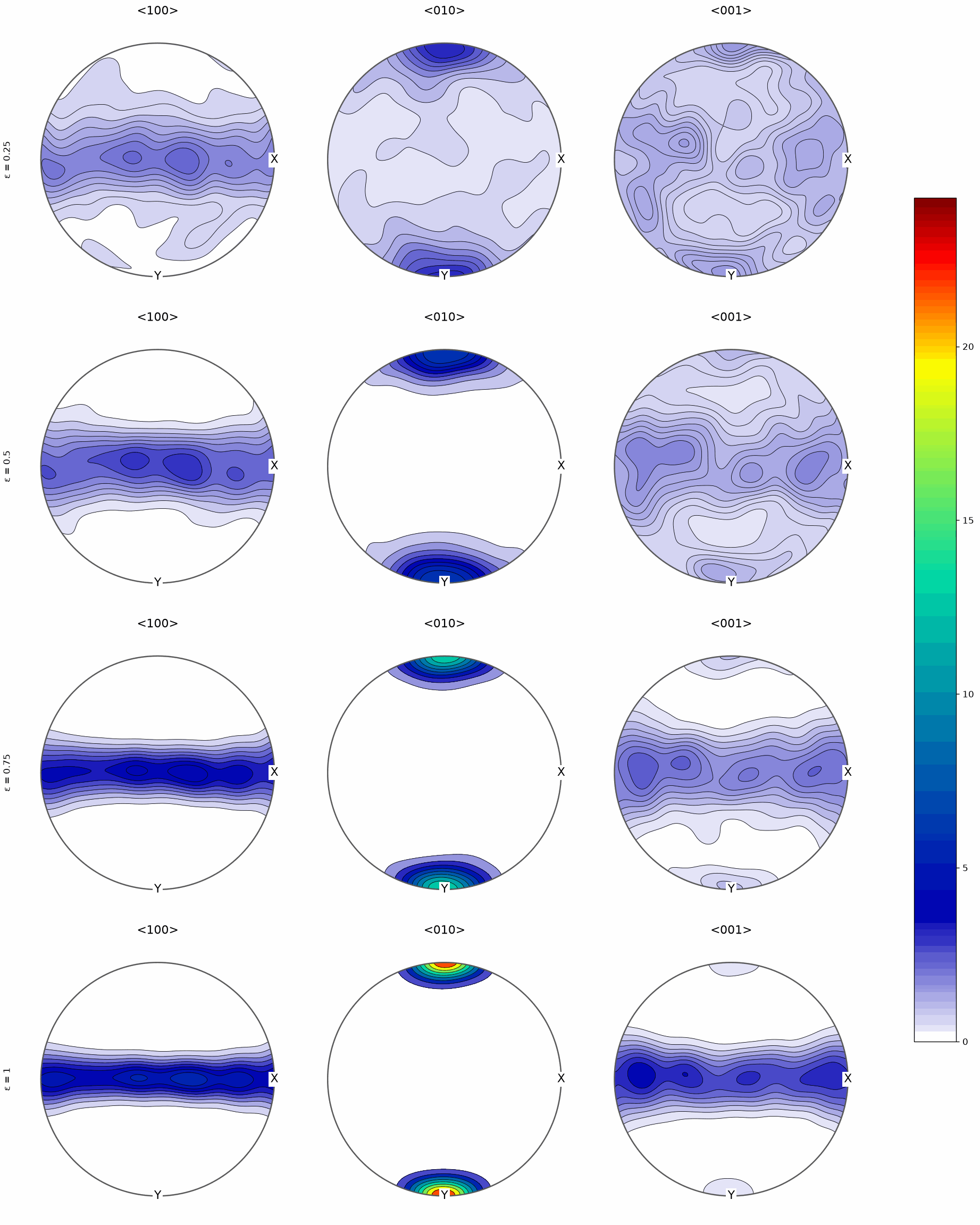
Read the rows from top to bottom as strain increases from 0.25 to 1.00. The shared colour range makes intensities comparable between rows; the changing peak positions and strengths are therefore texture evolution, not independent plot scaling.

Visualize slip-system activity

VPSC also writes ACT_PH1.OUT alongside the orientation data. It contains the activity of the different slip modes during deformation. Read it as a table with named columns so its STRAIN and MODE1 through MODE9 columns retain their names.

ACT = np.genfromtxt(os.path.join(path2file, 'ACT_PH1.OUT'), names=True)
print(' '.join(f'{n:>6}' for n in ACT.dtype.names))
for row in ACT:
  print(' '.join(f'{v:6.3f}' for v in row))

STRAIN  AVACS  MODE1  MODE2  MODE3  MODE4  MODE5  MODE6  MODE7  MODE8  MODE9
 0.000  2.835  0.337  0.310  0.309  0.011  0.012  0.007  0.003  0.002  0.009
 0.250  2.766  0.312  0.230  0.417  0.009  0.010  0.007  0.005  0.003  0.009
 0.500  2.835  0.317  0.198  0.445  0.007  0.009  0.007  0.007  0.004  0.006
 0.750  2.825  0.310  0.131  0.513  0.005  0.007  0.006  0.015  0.007  0.006
 1.000  2.759  0.312  0.075  0.554  0.003  0.005  0.006  0.028  0.013  0.005
 1.250  2.746  0.327  0.053  0.546  0.002  0.004  0.005  0.041  0.020  0.002
 1.500  2.736  0.370  0.048  0.521  0.002  0.005  0.005  0.033  0.015  0.002
 1.750  2.739  0.394  0.046  0.503  0.002  0.005  0.005  0.031  0.013  0.003
 2.000  2.828  0.435  0.048  0.468  0.002  0.005  0.004  0.025  0.009  0.004

Plot every mode against strain. AVACS is the second column and is not a slip mode, so the loop begins at the third column.

plt.figure(figsize=(9, 4.5))
for n, name in enumerate(ACT.dtype.names[2:], start=1):
  plt.plot(ACT['STRAIN'], ACT[name], linewidth=2, label=f'Slip mode {n}')

plt.xlabel('Strain')
plt.ylabel('Slip activity')
plt.legend(loc='upper left', bbox_to_anchor=(1, 1))
plt.ylim(-0.005, 1)
plt.tight_layout()

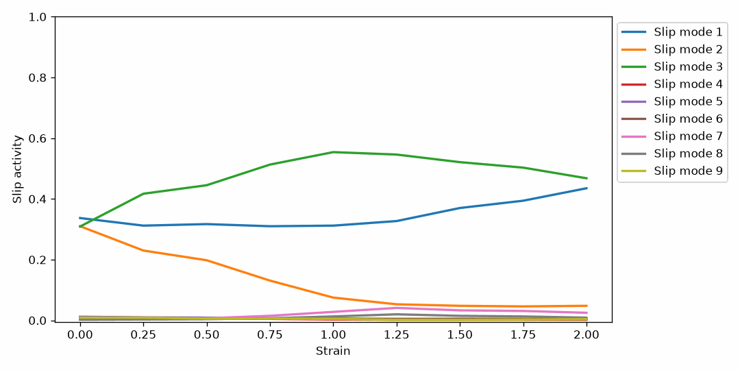
Modes 1-3 dominate this simulation. Mode 3 rises to its maximum near strain 1, mode 2 steadily weakens, and mode 1 nearly catches mode 3 at the final step. To inspect a single mode as a smooth curve, for example mode 3, one can fit scipy.interpolate.CubicSpline(ACT['STRAIN'], ACT['MODE3']) and plot it.

References

• R. A. Lebensohn and C. N. Tomé, A self-consistent anisotropic approach for the simulation of plastic deformation and texture development of polycrystals, Acta Metallurgica et Materialia 41 (1993), 2611-2624. This paper introduces the VPSC formulation used to compute the imported deformation history.

Next

Texture Evolution rotates every orientation by the Taylor-model spin over small strain increments. It provides the next step when the texture path should be computed inside MTEX rather than imported from VPSC.

@article{bachmann2010mtex,
  author  = {F. Bachmann and R. Hielscher and H. Schaeben},
  title   = {Texture Analysis with MTEX - Free and Open Source Software Toolbox},
  journal = {Solid State Phenomena},
  volume  = {160},
  pages   = {63-68},
  year    = {2010},
  doi     = {10.4028/www.scientific.net/SSP.160.63},
  url     = {https://doi.org/10.4028/www.scientific.net/SSP.160.63}
}