
encode two scalar properties as hue × saturation colors
Description
The first property selects the hue, sampled from a colour map, the second the saturation, from no colour (white or black) to the full colour:
* property 1 - hue, sampled from a user-supplied or the default colour map
* property 2 - saturation, linearly from white or black to the full colour
Syntax
cK = planarColorKeyKey over the default colour map.
cK = planarColorKey(winter,'shading','black')Key over winter, fading to black.
rgb = cK.property2color(v1, v2)Colours of the values v1, v2.
plot(cK)Standalone legend (key image only, no labels).
plot(cK, v1, v2)Legend with axes and labels according to the data range.
Input
| winter | n x 3 colour map of the hue, or the name of one |
| v1 | double, the property mapped to hue |
| v2 | double, the property mapped to saturation, same size as v1 |
Options
| shading | 'white' (default) or 'black', what zero saturation maps to |
| satRange | saturation range for v2, default [0 1] |
| quantileCap | quantile for the maximum of v2, default 0.975 |
| range1 | data range of v1, default [min(v1), max(v1)] |
| range2 | data range of v2, default [min(v2), quantile(v2,0.975)] |
| label1 | x-axis label in plot(), default 'Property 1' |
| label2 | y-axis label in plot(), default 'Property 2' |
Output
| cK | planarColorKey |
| rgb | colours of size [size(v1), 3] |
Class Properties
| colorMap | n x 3 hue look-up table |
| shading | 'white' (default) or 'black', what zero saturation maps to |
| satRange | saturation range for v2 |
| periode | period of periodic data (pi or 2*pi), wrapping v1, default NaN |
| quantileCap | quantile for the maximum of v2 |
| range1 | data range of v1 |
| range2 | data range of v2 |
| label1 | x-axis label in plot() |
| label2 | y-axis label in plot() |
Example
Example 1: long axis mapping, with saturation given by aspect ratio get the data
mtexdata martensite silent
grains = ebsd('indexed').calcGrains('minPixel',5);
asr  = grains('indexed').aspectRatio;
lax  = grains('indexed').longAxis;
set up colormap
pK = planarColorKey(colorcet('C2'));
% since long axis direction is periodic and antipodal (=pi)
pK.periode = pi;
pK.label1 = 'phi';
pK.label2 = 'a/b';
% and plot it
plot(pK,mod(lax.rho,pi)/degree,asr)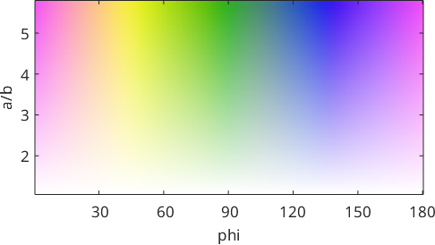
use the key to colorize the map
plot(grains('indexed'),pK.property2color(mod(lax.rho,pi)/degree,asr))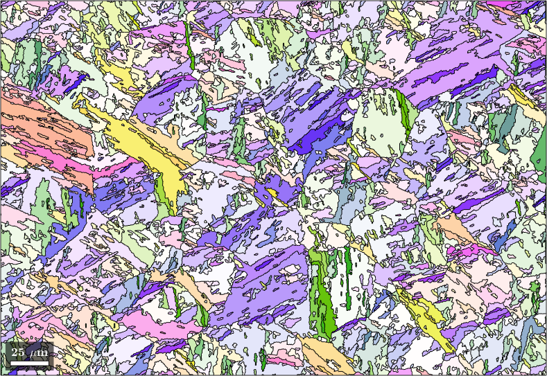
example 2: highlight grains which are large AND have a large aspect ratio
v1 = grains('indexed').aspectRatio;
v2 = grains('indexed').area;
set a colormap
pK = planarColorKey(inferno);shade to black
pK.shading = 'black';set the range1 for v1
pK.range1 = [1 4];set the autoselection of v2 a little lower
pK.quantileCap = 0.9;set labels
pK.label1 = 'asr'; pK.label2 = 'area';
close all; plot(pK,v1,v2)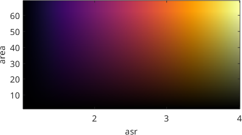
plot(grains('indexed'),pK.property2color(v1,v2))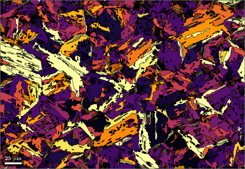
See also
Citing this page.
This page is part of the documentation of
MTEX, a free and open
source MATLAB toolbox for analyzing and modeling crystallographic textures.
It was written by The MTEX Developers and is published at
https://mtex-toolbox.github.io/planarColorKey.html.
If you use MTEX, or reuse text or figures from this page, in your research,
please cite
F. Bachmann, R. Hielscher, H. Schaeben: Texture Analysis with MTEX - Free and Open Source Software Toolbox, Solid State Phenomena 160 (2010), 63-68. 10.4028/www.scientific.net/SSP.160.63
BibTeX
@article{bachmann2010mtex,
  author  = {F. Bachmann and R. Hielscher and H. Schaeben},
  title   = {Texture Analysis with MTEX - Free and Open Source Software Toolbox},
  journal = {Solid State Phenomena},
  volume  = {160},
  pages   = {63-68},
  year    = {2010},
  doi     = {10.4028/www.scientific.net/SSP.160.63},
  url     = {https://doi.org/10.4028/www.scientific.net/SSP.160.63}
}
Other papers describing specific MTEX methods are listed under Publications — please cite the one that best fits your application. The MTEX source code is licensed under the GNU General Public License v2.0; the text and figures of this documentation are licensed under CC BY 4.0, which permits reuse — including by automated systems — provided The MTEX Developers and this page are credited.