
estimate a smooth density from orientations, directions, angles or real-valued samples.
Syntax
odf = calcDensity(ori)
Select the smoothing width from the orientations.
odf = calcDensity(ori, halfwidth=5*degree)
Use a fixed angular halfwidth.
odf = calcDensity(ori, kernel=SO3AbelPoissonKernel(halfwidth=10*degree))
Choose another kernel family.
odf = calcDensity(grains.meanOrientation, weights=grains.area)
Weight each grain by its area.
odf = calcDensity(ebsd)
Use a single-phase map with grain ids.
odf = calcDensity(ori, harmonic=True, bandwidth=16)
Return a harmonic expansion through degree 16.
sF = calcDensity(v, halfwidth=10*degree, weights=w)
Estimate a weighted directional density.
sF = calcDensity(v, halfwidth=10*degree, antipodal=True)
Treat opposite directions as the same axis.
f = calcDensity(rho, periodic=True, sigma=5*degree)
Estimate a density of angles on the circle.
f = calcDensity(x, range=[0, 1])
Estimate a density of real values on an interval.
f = calcDensity(X, range=[[0, 0], [1, 1]], rng=rng)
Estimate a joint density from rows of (x, y) samples.
Description
The estimate replaces the sample cloud with a smooth function. Narrow kernels retain finer detail; wider kernels suppress more sampling noise. Use odf(oriQuery), sF(vQuery) or f(xQuery) to evaluate it. For a joint density in two dimensions, use f(xQuery, yQuery); the coordinate arrays broadcast together.
The input determines the domain and the meaning of the density:
| Input | Estimate | Normalisation |
|---|---|---|
| orientation or rotation | orientation distribution function (ODF) on SO(3) | mean one; a value of two is twice the uniform density |
| vector3d or Miller | density of directions or axes on the sphere | mean one, with the input’s frame symmetry |
| numeric angles with periodic=True | density on the circle, with period 2*pi | mean one, with angles in radians |
| numeric array without circular options | density of real values, one sample per row | probability density in the units of the data |
For orientations and directions, an explicit halfwidth uses a de la Vallee Poussin
kernel; halfwidth is the angle at which the kernel falls to half its peak. Without a
halfwidth or kernel, calcKernel selects the width by unbiased cross validation with
a noise floor. Angular halfwidths are in radians; write 5*degree for five degrees.
For an EBSD map, select one phase before calling. Its grain ids are used automatically when available, so neighbouring pixels within a grain are grouped during width selection. Map orientations without grain groups use a halfwidth of 10 degrees and issue a warning. Automatic selection also falls back to 10 degrees when it cannot be performed, for example with fewer than two valid points. NaN orientations and directions are omitted; if none remain, their density is uniform. These empty-sample rules do not apply to numeric angles or real-valued data.
Numeric arrays are interpreted as real-valued data by default. Use periodic=True for angles; supplying sigma, kernel or antipodal also selects the circle estimator, even when antipodal=False. Circular data use a Gaussian kernel with Silverman’s width rule unless sigma or kernel is supplied. Real-valued data use a diffusion estimate in one dimension and a fitted Gaussian mixture in several dimensions.
Additional options depend on the input. Omitted weights give every sample equal weight; supplied weights are normalised internally.
| Option | Meaning and default |
|---|---|
| halfwidth | orientations, directions: angular kernel halfwidth in radians; selected automatically if neither halfwidth nor kernel is given |
| kernel | orientations, directions, angles: SO3Kernel, S2Kernel or S1Kernel matching the domain; takes precedence over halfwidth or sigma |
| weights | orientations, directions, angles, one-dimensional real data: one nonnegative weight per sample, with a positive total |
| groups | orientations, directions: one group id per sample for automatic width selection; groups are treated as independent units |
| antipodal | directions, angles: identify v with -v, or rho with rho+pi; default False, while axes already marked on vector3d remain axes |
| harmonic | orientations: True returns SO3FunHarmonic; False keeps the kernel sum as SO3FunRBF; by default use harmonics above 200 orientations when the kernel bandwidth is at most 96, with a Dirichlet kernel, or when both frames are crystal frames |
| bandwidth | orientations, directions, angles: maximum harmonic degree, controlling expansion resolution rather than the smoothing width; defaults depend on the kernel and MTEX bandwidth preferences |
| bandwidth | one-dimensional real data: Gaussian smoothing width in the units of the data; selected automatically by default |
| periodic | numeric angles: True selects the circular estimator; default False |
| sigma | numeric angles: standard deviation of the wrapped Gaussian in radians; selected by Silverman’s rule by default |
| range | real-valued data: [lo, hi] in one dimension, or [minima, maxima] with one column per dimension; defaults to the data’s bounding box |
| rng | multidimensional real data: numpy.random.Generator for the Gaussian mixture’s random initialisation; a new generator by default |
Multidimensional real data currently ignore weights and bandwidth. For orientations,
bandwidth is used when the estimate is built with harmonic=True; Fourier=True converts
the result to harmonics afterwards. Use harmonic=True to request a specific degree.
MATLAB’s ‘order’ is bandwidth; for a Bingham model use calcBinghamODF.
Input
x |
orientations or rotations, directions or Miller indices, a single-phase EBSD map, an array of angles, or a real array of shape (n,) or (n, d) |
Keywords
| keyword | default | description |
|---|---|---|
Fourier |
False |
convert the orientation density to SO3FunHarmonic after estimation; has no effect for other input types; MATLAB’s flag ‘Fourier’ |
Output
f |
callable density: SO3FunRBF or SO3FunHarmonic for orientations, S2FunHarmonic for directions, S1FunHarmonic for angles, or griddedDensity for real-valued data |
Example
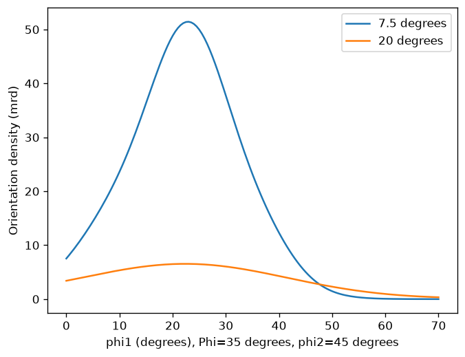
Estimate an orientation density from a reproducible synthetic sample. Compare two angular halfwidths along one Euler-angle section through the density.
import numpy as np
import matplotlib.pyplot as plt
from mtex import crystalFrame, orientation, calcDensity, degree

rng = np.random.default_rng(7)
cs = crystalFrame('m-3m')
angles = rng.normal([25, 35, 45], [8, 8, 8], size=(80, 3)) * degree
ori = orientation.byEuler(angles, cs)
narrow = calcDensity(ori, halfwidth=7.5*degree)
broad = calcDensity(ori, halfwidth=20*degree)
phi1 = np.linspace(0, 70, 141)
probe = orientation.byEuler(phi1*degree, 35*degree, 45*degree, cs)
plt.plot(phi1, narrow(probe), label='7.5 degrees')
plt.plot(phi1, broad(probe), label='20 degrees')
plt.xlabel('phi1 (degrees), Phi=35 degrees, phi2=45 degrees')
plt.ylabel('Orientation density (mrd)')
plt.legend()
print('Mean orientation density:', round(float(narrow.mean()), 3))
plt.show()
The broader kernel smooths more strongly. Both ODFs have mean one over orientation space; this one-dimensional section is not itself a probability density normalized to area one. Numeric real-valued inputs to calcDensity instead return a probability density in data units.
Mean orientation density: 1.0
See also
calcKernel, calcBinghamODF, unimodalODF, interpolate, calcDensityReal, DensityEstimation
Used on
EBSD2ODF, EBSDAdvancedMaps, EBSDOrientationAnalysis, CPOSeismicProperties, DensityEstimation, OptimalKernel, CSLBoundaries, SubGrainBoundaries, TiltAndTwistBoundaries, EllipseBasedParameters, GrainOrientationParameters, Grain_dispersion_axes
MATLAB’s calcDensity
source
Citing this page.
This page is part of the documentation of
MTEX, a free and open
source MATLAB toolbox for analyzing and modeling crystallographic textures.
It was written by The MTEX Developers and is published at
https://mtex-toolbox.github.io/calcDensity_py.html.
If you use MTEX, or reuse text or figures from this page, in your research,
please cite
F. Bachmann, R. Hielscher, H. Schaeben: Texture Analysis with MTEX - Free and Open Source Software Toolbox, Solid State Phenomena 160 (2010), 63-68. 10.4028/www.scientific.net/SSP.160.63
BibTeX
@article{bachmann2010mtex,
  author  = {F. Bachmann and R. Hielscher and H. Schaeben},
  title   = {Texture Analysis with MTEX - Free and Open Source Software Toolbox},
  journal = {Solid State Phenomena},
  volume  = {160},
  pages   = {63-68},
  year    = {2010},
  doi     = {10.4028/www.scientific.net/SSP.160.63},
  url     = {https://doi.org/10.4028/www.scientific.net/SSP.160.63}
}
Other papers describing specific MTEX methods are listed under Publications — please cite the one that best fits your application. The MTEX source code is licensed under the GNU General Public License v2.0; the text and figures of this documentation are licensed under CC BY 4.0, which permits reuse — including by automated systems — provided The MTEX Developers and this page are credited.