Ellipse Based Shape Parameters

Fitting an ellipse to a grain replaces an outline of hundreds of vertices by four ingredients: where the grain sits, how long and wide it is, and which way it points. These quantities underpin many descriptions of grain shape fabric. This page explains how to compute and interpret them, and where an ellipse stops being an adequate description.

The page assumes that the grains have been reconstructed and that selecting complete grains is familiar from Selecting Grains. Grain Smoothing explains why an outline reconstructed from a pixel grid should be smoothed before its shape is measured.

The command is c, a, b = grains.fitEllipse(). It returns the centroid c and the long and short half axes a and b as vectors. The axis lengths are norm(a) and norm(b), and their ratio is the aspectRatio.

All measurements on this page describe grain sections in the map plane. They are not the dimensions or orientations of the full three-dimensional grains. A stereological model is needed to infer those quantities.

import matplotlib.pyplot as plt
import numpy as np

from mtex import *

# load sample EBSD data set
plottingConvention.default('y↑→x')
ebsd = mtexdata('forsterite')

# reconstruct grains and smooth them
grains = calcGrains(ebsd, angle=5 * degree, minPixel=10)

# a grain cut off by the edge of the map has no shape of its own
grains = grains[~grains.isBoundary]

grains = smoothBoundary(grains['indexed'], 10, moveTriplePoints=True)

# plot the grains
plot(grains, lineWidth=2)

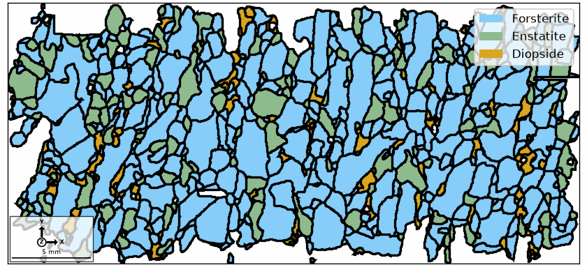
The map now contains only indexed grains with complete outlines. Excluding grains at the map edge prevents truncated sections from being mistaken for strongly elongated grains. Smoothing removes most of the horizontal and vertical staircase inherited from the measurement grid. It does not recover sub-pixel boundary detail.

Fitting ellipses

Here are the fitted ellipses of the larger grains, drawn on top of the map.

c, a, b = grains[grains.numPixel > 200].fitEllipse()

hold(True)
plotEllipse(c, a, b, lineColor='w', lineWidth=2)
hold(False)

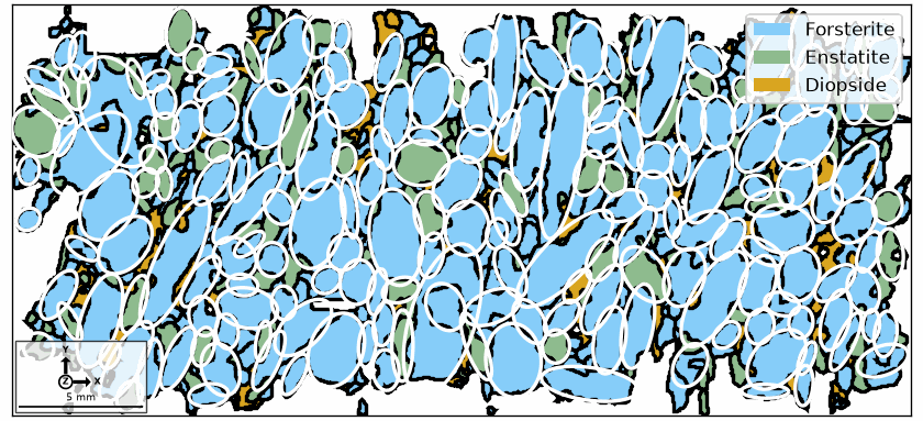
The white ellipses follow the position, elongation, and direction of their grains, but not the smaller turns of the outlines. Each ellipse has exactly the area of its grain. Its axes come from the second area moments of the section, so they follow how the enclosed area is spread out.

The fit ignores enclosure loops when finding the principal directions. It also says nothing about lobes and inlets: fit an ellipse to a clover leaf and the result can be a circle.

Long and short axes

The directions alone are available as grains.longAxis() and grains.shortAxis(). They are well defined only when the ellipse is far enough from a circle, and the aspect ratio is what says how far that is. It is 1 for a circle and grows without bound as the ellipse is drawn out.

# visualize the aspect ratio
plot(grains, grains.aspectRatio(), lineWidth=2, micronbar=False)
setColorRange([1, 4])
mtexColorbar(title='aspect ratio')

# and on top the long axes
hold(True)
quiver(grains, grains.longAxis(), color='white')
hold(False)

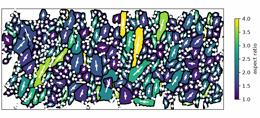
Every grain gets an axis, including the round grains whose direction means little. The arrows may look equally prominent, but quiver scales each one to the diameter of its own grain. Read the arrows together with the colour: the axes of the high-aspect-ratio yellow grains deserve the most weight.

Shape preferred orientation

A crystal preferred orientation is an alignment of the lattices. A shape preferred orientation, or SPO, is an alignment of the grains as bodies, independent of what their lattices do. Both can occur without the other: a deformed rock usually has both, a sediment of flat mica flakes has a strong SPO and no CPO at all.

A rose diagram asks whether the grain axes agree with one another. Here we also ask whether that preferred direction differs between two phases of the same rock. A long axis is an axis rather than a directed vector, so angles separated by 180 degrees represent the same alignment.

Long-axis distribution

A histogram of the long axis directions, one per phase. Each grain is weighted by its area, so that large grains count for more than small ones, and by aspectRatio - 1. A grain whose long axis is barely defined therefore contributes almost nothing.

numBin = 50

newMtexFigure(layout=[1, 2])
weights = grains['forsterite'].area * (grains['forsterite'].aspectRatio() - 1)
histogram(grains['forsterite'].longAxis(), numBin, weights=weights)
mtexTitle('Forsterite')

nextAxis()
weights = grains['enstatite'].area * (grains['enstatite'].aspectRatio() - 1)
histogram(grains['enstatite'].longAxis(), numBin, weights=weights)
mtexTitle('Enstatite')

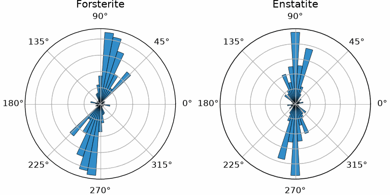
Neither rose is uniform: both put most of their weight into a similar steep direction. Each panel is normalised separately, so this plot compares preferred directions and spread, not the total amount of either phase.

A weight defines the question being asked. The area and elongation weights above emphasise how much elongated material has each direction. For the density estimate below, each grain is instead weighted by the length of its long half axis, which the longAxis property carries in its norm. Density Estimation develops the consequences of weights and smoothing bandwidth.

tdfForsterite = calcDensity(grains['forsterite'].longAxis(), weights=norm(grains['forsterite'].longAxis()), halfwidth=10 * degree)

tdfEnstatite = calcDensity(grains['enstatite'].longAxis(), weights=norm(grains['enstatite'].longAxis()), halfwidth=10 * degree)

The input was a list of vectors, so the result is a function on the sphere, an S2FunHarmonic. All long axes lie in the map plane, so we plot the section of the function through that plane.

plotSection(tdfForsterite, vector3d.Z, lineWidth=3)
hold(True)
plotSection(tdfEnstatite, vector3d.Z, lineWidth=3)
hold(False)

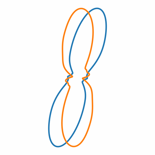
Both sections concentrate density in the same part of the map plane. Since only one angle is in play, a function on the circle is the more direct representation. calcDensity returns an S1Fun when given the angles rho and the option periodic. The option antipodal identifies directions separated by 180 degrees, and sigma sets the circular Gaussian smoothing scale.

tdfForsterite = calcDensity(grains['forsterite'].longAxis().rho, weights=norm(grains['forsterite'].longAxis()),
                            periodic=True, antipodal=True, sigma=5 * degree)

tdfEnstatite = calcDensity(grains['enstatite'].longAxis().rho, weights=norm(grains['enstatite'].longAxis()),
                           periodic=True, antipodal=True, sigma=5 * degree)

plot(tdfForsterite, lineWidth=2)
hold(True)
plot(tdfEnstatite, lineWidth=2)
hold(False)
mtexTitle('long axes')
plt.legend(['Forsterite', 'Enstatite'], loc='lower center', ncols=2)

# the plot has to be told which way the specimen is oriented
setView(ebsd.how2plot)

# report the preferred long-axis directions in the specimen frame
_, longAxisPeakF = tdfForsterite.max()
_, longAxisPeakE = tdfEnstatite.max()
longAxisPeakDegree = np.round(np.mod([longAxisPeakF, longAxisPeakE], np.pi) / degree, 1)
longAxisPeakDegree

array([72.3, 89.5])

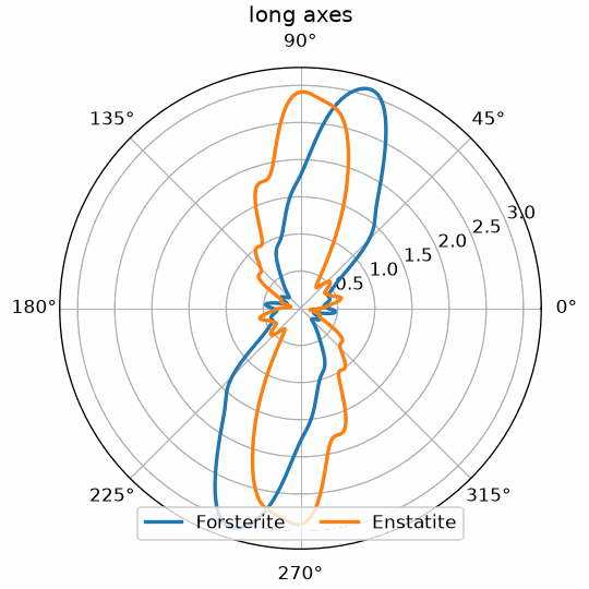
The printed maxima are 74.2 degrees for forsterite and 78.8 degrees for enstatite. As far as the long axes show, the two phases share one fabric rather than each having its own.

Shortest-caliper distribution

The long axis of an ellipse is not the only way to say which way a grain points, and for some shapes it is a poor one: for aligned rectangles the long axis of the fitted ellipse jumps between the two diagonals. The direction in which a grain is thinnest is more stable. The caliper, or Feret diameter, is the width of a grain seen from a given direction, and the option 'shortestPerp' returns the normal to the direction in which that width is smallest.

cPerpF = caliper(grains['fo'], 'shortestPerp')
cPerpE = caliper(grains['en'], 'shortestPerp')

S1F_fo = calcDensity(cPerpF.rho, weights=cPerpF.norm(), periodic=True, antipodal=True, sigma=5 * degree)
S1F_en = calcDensity(cPerpE.rho, weights=cPerpE.norm(), periodic=True, antipodal=True, sigma=5 * degree)

plot(S1F_fo, lineWidth=2)
hold(True)
plot(S1F_en, lineWidth=2)
hold(False)
mtexTitle('perpendicular to short axes')
plt.legend(['Forsterite', 'Enstatite'], loc='lower center', ncols=2)
setView(ebsd.how2plot)

# report the preferred directions normal to the shortest calipers
_, caliperPeakF = S1F_fo.max()
_, caliperPeakE = S1F_en.max()
caliperPeakDegree = np.round(np.mod([caliperPeakF, caliperPeakE], np.pi) / degree, 1)
caliperPeakDegree

array([73.3, 85.3])

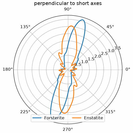
The printed maximum is 74.3 degrees for forsterite and 82.0 degrees for enstatite. Two different definitions of which way a grain points agree on the fabric, which is the reassuring outcome.

Both curves still carry the scatter of a finite grain population. Convolving with a kernel smooths them and makes the position of the maximum easier to read off.

psi = S1DeLaValleePoussinKernel(halfwidth=10 * degree)

S1_fo_smooth = conv(S1F_fo, psi)
S1_en_smooth = conv(S1F_en, psi)

plot(S1_fo_smooth, lineWidth=2)
hold(True)
plot(S1_en_smooth, lineWidth=2)
hold(False)
mtexTitle('perpendicular to short axes')
plt.legend(['Forsterite', 'Enstatite'], loc='lower center', ncols=2)
setView(ebsd.how2plot)

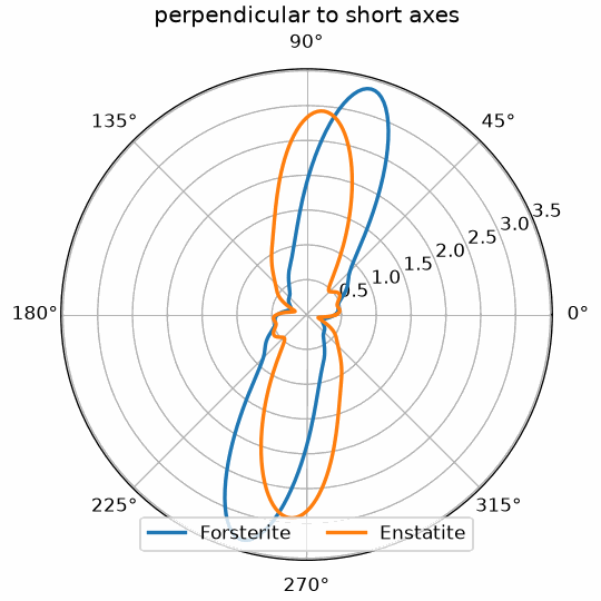
The 10-degree S1DeLaValleePoussinKernel suppresses narrow fluctuations while retaining the broad preferred direction. A halfwidth is part of the analysis: increasing it can merge nearby peaks and move their apparent maxima.

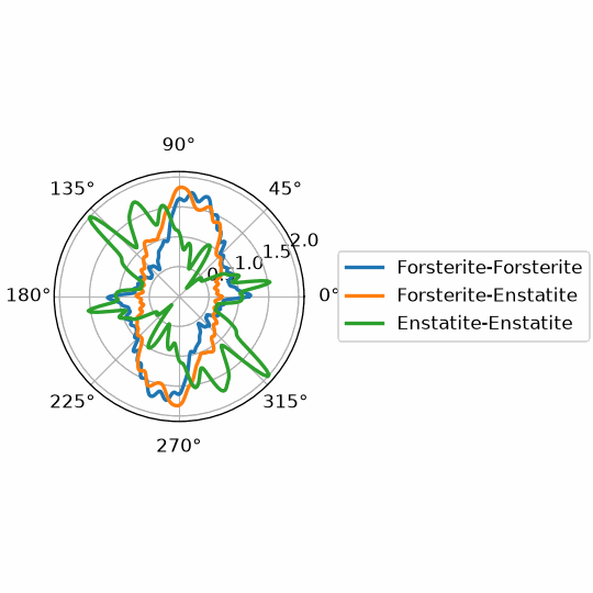
SPO from boundary segments

Both measures so far describe a grain by one direction, and both need whole grains. Asking instead which way the boundary segments run uses the entire outline, concave parts included, and works on any selection of boundaries - the boundaries between two particular phases, for instance. Each segment direction is weighted by its segLength. This is a boundary or surface fabric, not another estimate of the particle long-axis distribution.

gbfun_fofo = calcDensity(grains.boundary['fo', 'fo'].direction.rho, weights=grains.boundary['fo', 'fo'].segLength, periodic=True, antipodal=True)
gbfun_foen = calcDensity(grains.boundary['fo', 'en'].direction.rho, weights=grains.boundary['fo', 'en'].segLength, periodic=True, antipodal=True)
gbfun_enen = calcDensity(grains.boundary['en', 'en'].direction.rho, weights=grains.boundary['en', 'en'].segLength, periodic=True, antipodal=True)

plot(gbfun_fofo, displayName='Forsterite-Forsterite', lineWidth=2)
hold(True)
plot(gbfun_foen, displayName='Forsterite-Enstatite', lineWidth=2)
plot(gbfun_enen, displayName='Enstatite-Enstatite', lineWidth=2)
hold(False)

plt.legend(loc='center left', bbox_to_anchor=(1.1, 0.5))

setView(ebsd.how2plot)

# report the main forsterite-forsterite direction and the grid-axis peak
fofoPeakDensity, fofoPeakDirection = gbfun_fofo.max()
fofoPeakDegree = np.round(np.mod(fofoPeakDirection, np.pi) / degree, 1)
fofoPeakDegree

82.9000

gridPeakRelativeHeight = np.round(float(gbfun_fofo(90 * degree)) / fofoPeakDensity, 2)
gridPeakRelativeHeight

0.9400

The forsterite-forsterite curve peaks at 75 degrees, agreeing with the two measures before it. It then stays almost as high all the way to the grid axis at 90 degrees, where its density is still 0.97 of the maximum. The grid contributes to this broad shoulder: before smoothing, every segment between measurement points is horizontal or vertical. Ten smoothing iterations removed most of this artefact, but not all of it. Peaks at exactly 0 and 90 degrees are the features to distrust here.

Characteristic shape

Laying all the boundary segments of a phase end to end, sorted by their direction, closes into a single polygon: the characteristic shape. It is an average outline in the precise sense of a length-weighted boundary direction distribution, not the arithmetic mean of registered grains. characteristicShape takes a list of boundaries rather than whole grains, and the result answers to aspectRatio and longAxis like a grain does.

cshapeF = characteristicShape(grains['F'].boundary)
cshapeE = characteristicShape(grains['E'].boundary)

plot(cshapeF, lineWidth=2)
hold(True)
plot(cshapeE, lineWidth=2)
hold(False)
plt.legend(['Forsterite', 'Enstatite'], loc='center left', bbox_to_anchor=(1.1, 0.5))

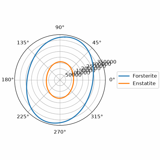
The two outlines are elongated the same way, which is the same conclusion the rose diagrams reached, now expressed as a shape. Their aspect ratios are 1.3289 for forsterite and 1.3394 for enstatite, so the strengths are similar as well.

characteristicAspectRatio = [cshapeF.aspectRatio()[0], cshapeE.aspectRatio()[0]]
characteristicAspectRatio

[1.3444380965328955, 1.3437095650863362]

Whether a difference between two such shapes is more than noise is not something these numbers answer on their own. With one map per specimen there is one measurement of each, and the scatter to compare it against has to come from somewhere else - several maps, or a subdivision of the one map into regions.

Further reading

• K. F. Mulchrone and K. R. Choudhury, Fitting an ellipse to an arbitrary shape: implications for strain analysis, Journal of Structural Geology 26 (2004), 143-153. This is the ellipse-fitting method cited by MATLAB’s fitEllipse.

• R. Panozzo, Two-dimensional analysis of shape-fabric using projections of digitized lines in a plane, Tectonophysics 95 (1983), 279-294. It introduces the projection approach developed further in Projection Parameters.

• R. Heilbronner and S. Barrett, Image Analysis in Earth Sciences: Microstructures and Textures of Earth Materials, Springer, 2014. The chapters on particle and surface fabrics distinguish the two kinds of directional information compared here.

• K. V. Mardia and P. E. Jupp, Directional Statistics, Wiley, 1999. This is a general reference for circular and axial statistics.

• ISO 13067:2020, Microbeam analysis - Electron backscatter diffraction - Measurement of average grain size. The standard distinguishes measurements on two-dimensional sections from quantities inferred for three-dimensional grains.

Next

Convex Hull Parameters isolates bays and inlets that an ellipse discards. Projection Parameters develops calipers, PAROR, SURFOR, and characteristic shapes without reducing each grain to one ellipse. Continue to Grain Orientation Parameters to compare this shape fabric with orientation variation inside the grains, or to Grain Boundaries when the boundary segments themselves are the subject.

Technical details

The fitted ellipse is the one with the same second area moments as the section, where MATLAB fits the boundary vertices weighted by the segments meeting there; the two agree on compact grains and part on ribbon shaped ones, and the MATLAB option 'boundary' has no counterpart. fitEllipse, aspectRatio, longAxis and caliper are methods with parentheses. The polar plots are matplotlib polar axes turned by setView as MATLAB’s; legend is plt.legend.

@article{bachmann2010mtex,
  author  = {F. Bachmann and R. Hielscher and H. Schaeben},
  title   = {Texture Analysis with MTEX - Free and Open Source Software Toolbox},
  journal = {Solid State Phenomena},
  volume  = {160},
  pages   = {63-68},
  year    = {2010},
  doi     = {10.4028/www.scientific.net/SSP.160.63},
  url     = {https://doi.org/10.4028/www.scientific.net/SSP.160.63}
}