Weighted Burgers Vector Analysis

The weighted Burgers vector (WBV) describes the net Burgers-vector content that crosses an EBSD section. Each dislocation line is weighted by the cosine of its angle to the map normal. Parallel Burgers vectors add, while opposing ones can cancel.

WBV analysis is complementary to, and can be used as an alternative to, geometrically necessary dislocation analysis. The GND workflow fits densities of chosen crystallographic systems. WBV analysis returns one vector without choosing systems, but it cannot by itself separate the contributing dislocation types or their cancelling densities.

weightedBurgersVec offers an integral method and a gradient method. This page computes both, shows their noise controls, and explains what their different spatial scales mean.

import numpy as np

from mtex import *

Prepare a single-grain map

Load the bundled single-phase aluminium map. Earlier wording called this the same data as the preceding GND example, but mtexdata('single') is a 101-by-101 aluminium map rather than the DC06 steel map used there.

ebsd = mtexdata('single')
ebsd

EBSD (y↓→x)
  size: 101 × 101 grid
  Phase  Orientations  Mineral  Color         Symmetry  Crystal reference frame
  1      10201 (100%)  Al       LightSkyBlue  m-3m      Al
  scan unit     : um
  X × Y         : [6 → 16] × [4 → 14]
  square lattice: spacing 0.1

Reconstruct grains because neither method should compare orientations across a grain boundary. Regions smaller than six pixels become notIndexed, as on the preceding page.

grains = calcGrains(ebsd, angle=2.5 * degree, minPixel=6)

# retain the unfiltered map for the window-size comparison
ebsdNoisy = ebsd.copy()

# denoise without smoothing across grain boundaries
F = halfQuadraticFilter()
ebsd = smooth(ebsd, F, fill=grains)

Integral method: compute the default WBV

The default integral method evaluates a square loop around every pixel. It uses a Prewitt-like convolution kernel whose four corner weights are one half. The default windowSize=1 gives a 3-by-3 loop.

A raster loop needs matrix-form data. This map is already gridded; a list of measurements is gridded first with gridify.

wbvIntegral = weightedBurgersVec(ebsd)
wbvIntegral

vector3d (y↓→x)
  size: 101 × 101
    x    y    z
  NaN  NaN  NaN
  NaN  NaN  NaN
  NaN  NaN  NaN
  NaN  NaN  NaN
  NaN  NaN  NaN
    ⋮    ⋮    ⋮
  NaN  NaN  NaN
  NaN  NaN  NaN
  NaN  NaN  NaN
  NaN  NaN  NaN
  NaN  NaN  NaN

The result is a vector3d at every EBSD pixel, expressed in the specimen frame. Its norm has units of inverse scan length, here \(1/\mathrm{\mu m}\).

plot(ebsd, wbvIntegral.norm(), refFrame='on')
mtexColorbar()
mtexTitle('WBV magnitude')

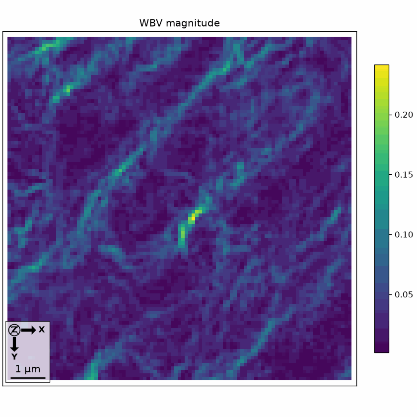
Bright pixels have a larger net Burgers-vector content through the local loop. A small norm does not prove that few dislocations are present, because vectors of opposite sign can cancel.

Show direction and magnitude together

A directional key assigns hue from vector direction. Opacity carries the norm, with values at and above 0.22 rendered fully opaque.

cK = HSVDirectionKey(wbvIntegral)
alphaIntegral = np.minimum(np.nan_to_num(wbvIntegral.norm()) / 0.22, 1)

newMtexFigure(layout=[1, 3], figSize='large')
plot(ebsd, cK.direction2color(wbvIntegral), faceAlpha=alphaIntegral)
mtexTitle('WBV in specimen coordinates')
nextAxis()
plot(cK, figSize='tiny')
mtexTitle('directional color key')

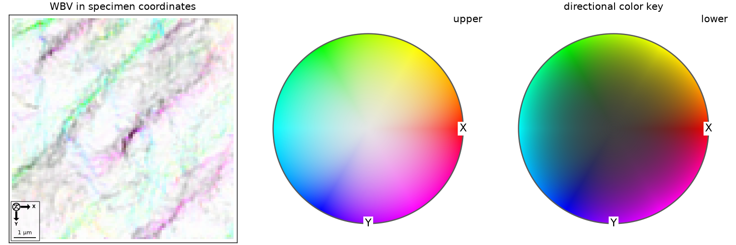
Read hue only where the map is sufficiently opaque. Hue in nearly transparent regions represents a poorly constrained direction of a small vector and should not dominate the interpretation.

Plot only the strongest vectors

Arrows at every pixel would hide the map. The 85th percentile is a display threshold, not a physical division between low and high dislocation content, so the arrows show only the strongest 15 percent of WBVs.

cond = wbvIntegral.norm() > np.nanquantile(wbvIntegral.norm(), 0.85)

newMtexFigure(layout=[1, 3], figSize='large')
plot(ebsd, cK.direction2color(wbvIntegral), faceAlpha=alphaIntegral)
hold(True)
quiver(ebsd[cond], wbvIntegral[cond], color='k', autoScaleFactor=2, antipodal=True, lineWidth=0.5)
hold(False)
mtexTitle('strongest WBVs in specimen coordinates')
nextAxis()
plot(wbvIntegral, weights=wbvIntegral.norm(), contourf=True)
mtexTitle('magnitude-weighted direction distribution')

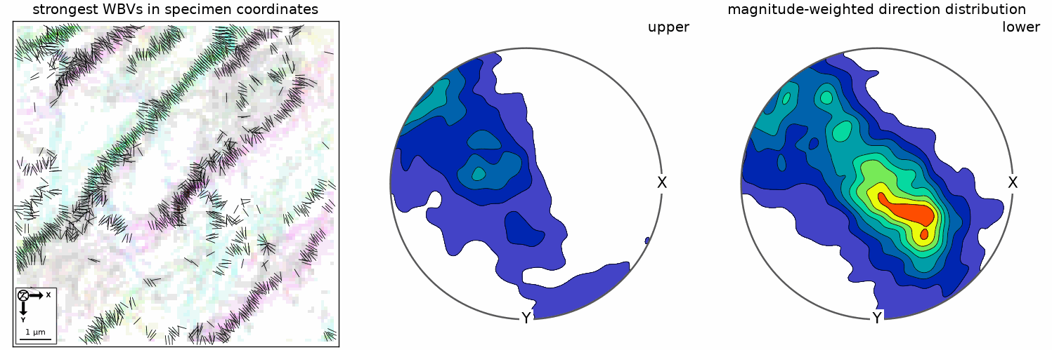
The arrows identify the local directions behind the map colors. The spherical plot summarizes those directions over the whole map, weighted by magnitude, so it does not preserve their spatial locations.

Express the WBV in each crystal frame

The same physical vector can be re-expressed in the crystal frame of each pixel by applying the inverse orientation. This is a frame change, not a rotation of the dislocation content.

wbvCrystal = inv(ebsd.orientations) * wbvIntegral
cKCrystal = HSVDirectionKey(wbvCrystal)

newMtexFigure(layout=[1, 2])
plot(ebsd, cKCrystal.direction2color(wbvCrystal), faceAlpha=alphaIntegral)
mtexTitle('WBV in crystal coordinates')
nextAxis()
plot(cKCrystal)
mtexTitle('directional color key')
hold(True)
plot(wbvCrystal, weights=wbvCrystal.norm(), contour=True, contours=np.arange(0.2, 2.01, 0.1), lineColor='k',
     contourLabels=True, lineWidth=2)
hold(False)

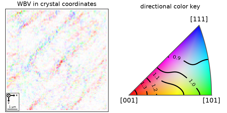
Directions that differ in the specimen frame can cluster in the crystal frame. The black contours show the magnitude-weighted direction density on the crystal-symmetry color key.

Increase the integral window

If denoising is undesirable, enlarge the loop instead. An integer windowSize=n selects a \((2n+1)\)-by-\((2n+1)\) loop, so the values 1, 2, and 3 below produce 3-by-3, 5-by-5, and 7-by-7 loops.

newMtexFigure(layout=[2, 4])
wbvDenoised = weightedBurgersVec(ebsd)
nextAxis(0, 0)
plot(ebsd, wbvDenoised.norm())
mtexTitle('denoised / box = 3')
nextAxis(1, 0)
plot(wbvDenoised, weights=wbvDenoised.norm(), contourf=True, antipodal=True)
mtexTitle('direction distribution')

for ws in [1, 2, 3]:
  wbvWindow = weightedBurgersVec(ebsdNoisy, windowSize=ws)
  nextAxis(0, ws)
  plot(ebsdNoisy, wbvWindow.norm())
  mtexTitle(f'noisy / box = {2 * ws + 1}')
  nextAxis(1, ws)
  plot(wbvWindow, weights=wbvWindow.norm(), contourf=True, antipodal=True)
  mtexTitle('direction distribution')

mtexColorbar()

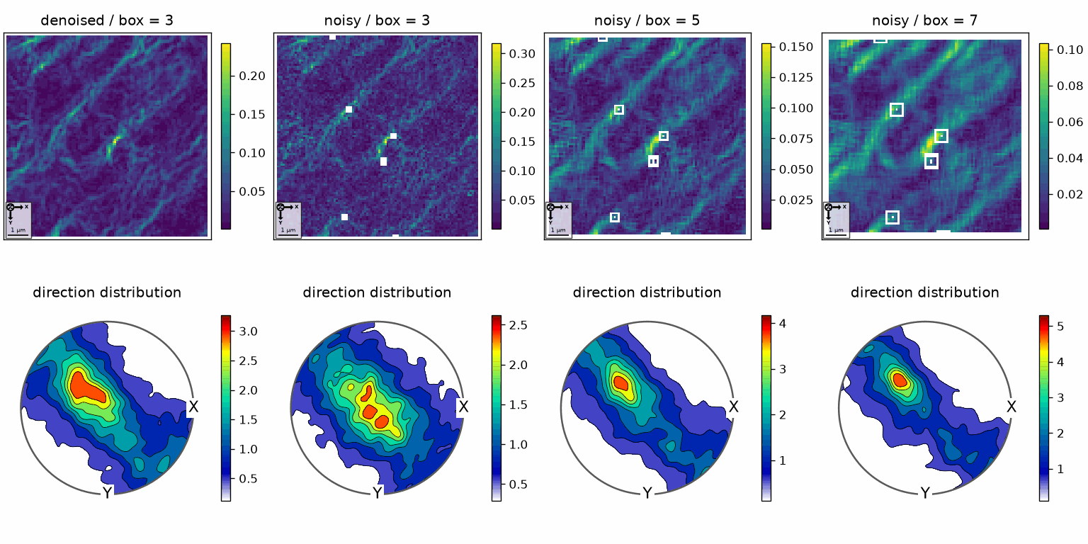
The noisy 3-by-3 result differs visibly from the denoised result. Larger loops suppress local scatter and sharpen the direction distribution, but they also spread sharp gradients and reduce the WBV norm.

Notice also the widening empty margins at the map border and around the unfilled points. A value is undefined wherever its loop crosses a point with no data, so increasing the window sacrifices both detail and coverage. A grain boundary interrupts a loop the same way; this map reconstructs to a single grain, so only the unfilled points do it here.

Gradient method

The gradient method takes the map-normal column of the dislocation-density tensor described on the preceding page. It resolves finer detail than a finite integration loop, but pointwise differentiation amplifies orientation noise. Use high-angular-resolution data or denoise the map first, as done here.

This method uses the virtual measurement lattice and does not require matrix-form data. It works on a plain EBSD map, a phase subset, and a rotated or sheared grid. The current implementation extracts the third Cartesian tensor column, so use it for a section whose normal is specimen \(z\). Earlier wording also claimed arbitrary non-\(xy\) sections; that case is not represented by the current extraction.

wbvGradientDefault = weightedBurgersVec(ebsd, gradient=True)

cKGradient = HSVDirectionKey(wbvGradientDefault)
plot(ebsd, cKGradient.direction2color(wbvGradientDefault),
     faceAlpha=np.minimum(np.nan_to_num(wbvGradientDefault.norm()) / 0.2, 1))
mtexTitle('gradient WBV in specimen coordinates')
nextAxis(0, 1)
plot(wbvGradientDefault, weights=wbvGradientDefault.norm(), antipodal=True, contourf=True)
mtexTitle('direction distribution')

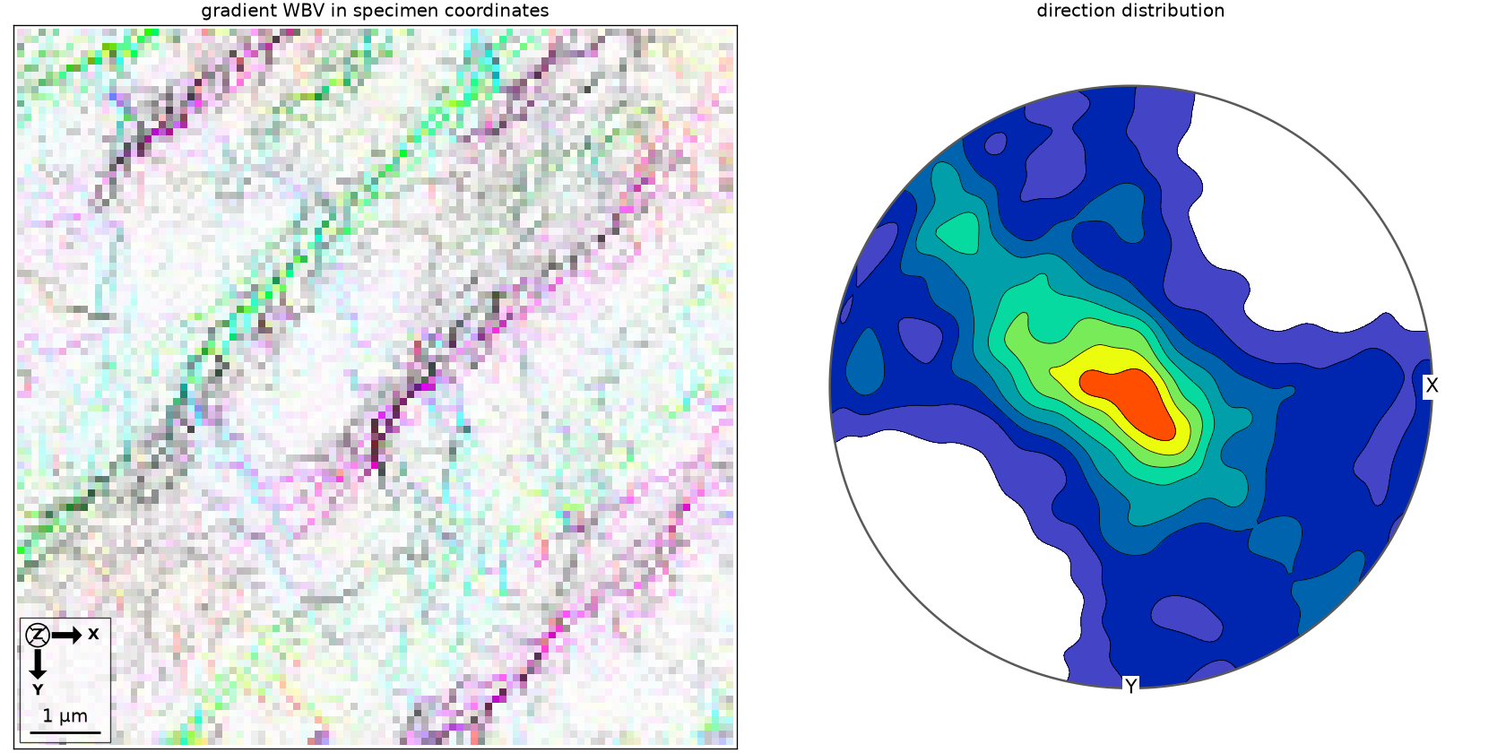
Compared with the denoised integral map, the gradient map retains sharper pixel-scale structures. Some of that extra detail may be noise, so the derivative stencil must be chosen with the spatial resolution in mind.

Choose the gradient stencil

The stencil option is passed to ebsd.gradient. All choices use only the immediate lattice neighbourhood, but trade locality against robustness.

• 'oneSided' is the default. It uses the neighbours in the positive two lattice directions and falls back to the opposite side at the map border. This forward difference is the most local and the most noise-sensitive.
• '1hop' fits a least-squares gradient over the lattice’s axial neighbours: four on a square grid and six on a hexagonal grid. In the interior of a square map this is the central difference.
• 'full' fits all eight surrounding pixels on a square grid, including the diagonals. It averages most and is best conditioned. A pixel needs two independent neighbour directions, so this stencil can also leave fewer undefined values on an interrupted map.

Where a map is broken up by notIndexed areas, phase boundaries, or grain boundaries, the three stencils differ in how many pixels they can still define. This map is dense and single-phase, so the difference here is only a couple of pixels at the border.

stencils = ['oneSided', '1hop', 'full']
wbvGradient = [weightedBurgersVec(ebsd, gradient=True, stencil=s) for s in stencils]

newMtexFigure(layout=[2, 3])
for k, s in enumerate(stencils):
  nextAxis(0, k)
  plot(ebsd, wbvGradient[k].norm(), micronbar='off')
  mtexTitle(f'WBV norm / {s}')
  nextAxis(1, k)
  plot(wbvGradient[k], weights=wbvGradient[k].norm(), contourf=True, antipodal=True)
  mtexTitle('direction distribution')
mtexColorbar()

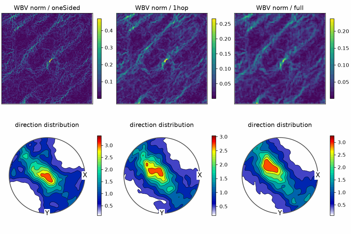
The three maps contain the same broad structures but become progressively smoother. The extrema expose the change better than the mean because the wider stencil averages the sharpest gradients first.

for s, wbvK in zip(stencils, wbvGradient):
  n = wbvK.norm()
  isDefined = ~np.isnan(n)
  print(f'{s:<9}  defined at {np.count_nonzero(isDefined)} of {n.size} pixels,  '
        f'mean |W| = {n[isDefined].mean():.4f},  max |W| = {n[isDefined].max():.4f}')

oneSided   defined at 10201 of 10201 pixels,  mean |W| = 0.0436,  max |W| = 0.4698
1hop       defined at 10201 of 10201 pixels,  mean |W| = 0.0367,  max |W| = 0.2673
full       defined at 10201 of 10201 pixels,  mean |W| = 0.0337,  max |W| = 0.2368

'oneSided' is defined at 10,198 of the 10,201 pixels and the other two at 10,200. The mean changes only from 0.0288 to 0.0271, while the maximum falls from 0.4340 to 0.2169, almost exactly by half. The stencil therefore acts most strongly on the sharpest gradients and leaves the bulk of this map comparatively stable.

Whether that change removes noise or erases structure is a question about the data. 'oneSided' preserves the most local features, 'full' is the most stable, and the symmetric '1hop' choice lies between them.

This control is distinct from integral windowSize. A stencil reaches only immediate neighbours; an integral loop can expand to 5-by-5, 7-by-7, and beyond. If 'full' does not sufficiently stabilize noisy data, denoise it or use a larger integral loop.

Why the two methods measure the same vector

If \(\boldsymbol\alpha\) is the Nye tensor and \(\mathbf n\) is the map normal, the weighted Burgers vector is

The second form shows the cosine weighting by line direction. The gradient method evaluates \(\boldsymbol\alpha\mathbf n\) locally. The integral method estimates the same net content from the orientation change around a finite loop, using a larger spatial support to reduce noise.

References

• J. Wheeler, D. J. Prior, Z. Jiang, R. Spiess and P. W. Trimby, The weighted Burgers vector: a new quantity for constraining dislocation densities and types using electron backscatter diffraction on 2D sections through crystalline materials, Journal of Microscopy 233 (2009), 482-494, introduces the WBV definition and its integral evaluation on EBSD sections.

Next

Continue with VPSC Import to bring the output of a viscoplastic self-consistent simulation into MTEX for texture analysis.

@article{bachmann2010mtex,
  author  = {F. Bachmann and R. Hielscher and H. Schaeben},
  title   = {Texture Analysis with MTEX - Free and Open Source Software Toolbox},
  journal = {Solid State Phenomena},
  volume  = {160},
  pages   = {63-68},
  year    = {2010},
  doi     = {10.4028/www.scientific.net/SSP.160.63},
  url     = {https://doi.org/10.4028/www.scientific.net/SSP.160.63}
}