Geometrically Necessary Dislocations

A spatial change in lattice orientation requires dislocations to preserve compatibility. These are geometrically necessary dislocations (GNDs). Conventional two-dimensional EBSD measures only the in-plane orientation gradient, so it cannot identify a unique three-dimensional dislocation population.

The workflow on this page follows Pantleon (2008). It computes the measured lattice curvature and fits the least-energy combination of candidate dislocation systems that reproduces it. Read Dislocation Systems first for the Burgers vector, line vector, tensor basis, and relative line-energy weights used here.

import numpy as np

from mtex import *

Load and segment the map

The example is a ferritic steel map after two percent uniaxial deformation. The minPixel option marks indexed regions smaller than six pixels as notIndexed during segmentation. A 2.5 degree threshold separates the remaining grains.

plottingConvention.default('y←↑x')
ebsd = mtexdata('dc06')

grains = calcGrains(ebsd, angle=2.5 * degree, minPixel=6)
grains = smoothBoundary(grains, 5)

An inverse pole figure (IPF) key colors each indexed orientation by the crystal direction parallel to specimen \(y\). The boundaries provide the spatial context for the orientation changes used below.

ipfKey = ipfHSVKey(ebsd)
ipfKey.ipfDirection = yvector

plot(ebsd, ipfKey.orientation2color(ebsd.orientations), refFrame='on', figSize='medium')
hold(True)
plot(grains.boundary, lineWidth=2)
hold(False)

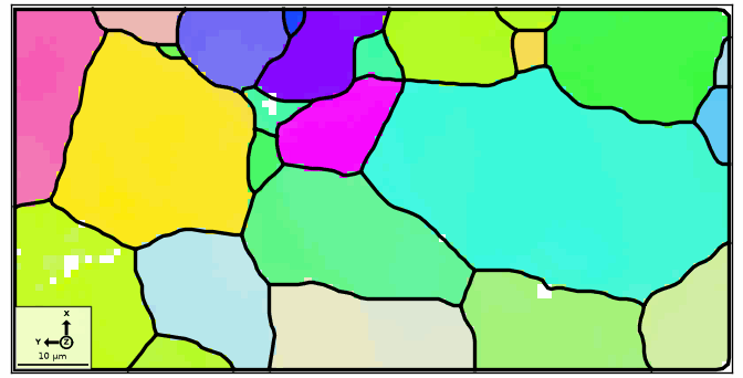
Notice that each grain has a dominant color, while smaller color changes remain inside many grains. Those intragranular changes carry the curvature signal, together with measurement noise.

Denoise before differentiating

Differentiation amplifies point-to-point orientation noise and therefore overestimates GND density. An axis-angle color key makes local departures from each grain’s mean orientation easier to see before filtering.

axisKey = axisAngleColorKey(ebsd)
axisKey.oriRef = grains['id', ebsd['indexed'].grainId].meanOrientation

plot(ebsd['indexed'], axisKey.orientation2color(ebsd['indexed'].orientations), micronbar='off', figSize='medium')
hold(True)
plot(grains.boundary, lineWidth=2)
hold(False)

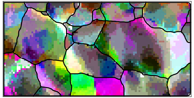
The pixel-scale color speckle is the symptom to notice. A halfQuadraticFilter reduces that noise while the fill option uses the grain partition to prevent smoothing across grain boundaries.

F = halfQuadraticFilter()
ebsd = smooth(ebsd, F, fill=grains)

axisKey.oriRef = grains['id', ebsd['indexed'].grainId].meanOrientation
plot(ebsd['indexed'], axisKey.orientation2color(ebsd['indexed'].orientations), micronbar='off', figSize='medium')
hold(True)
plot(grains.boundary, lineWidth=2)
hold(False)

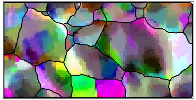
The denoised map retains broad color gradients inside grains but suppresses much of the isolated pixel-to-pixel variation. Filtering is therefore part of the measurement model, not merely cosmetic preparation for the plot.

Estimate GND content in one command

Ferrite is body-centred cubic, so this example uses the standard BCC set of 48 edge and 4 screw systems. Following the normalization on the preceding page, the line energies are taken relative to the shortest Burgers vector: the edge weight is one and the screw weight is \(1-\nu\), with Poisson’s ratio \(\nu=0.3\).

There is no universally accepted set of line-energy weights. Replace these illustrative values with values appropriate to the material and model.

dS = dislocationSystem.bcc(ebsd.CS)
nu = 0.3
dS.u = (dS.b.norm() / dS.b.norm().min()) ** 2 * (1 - nu * dS.isScrew)

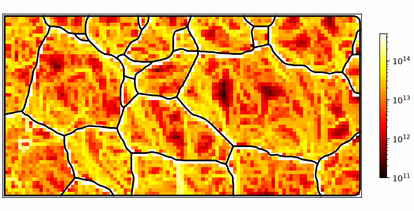
calcGND returns an energy-weighted GND density for each pixel and the signed density assigned to each candidate system. The first output is often called the total dislocation energy. With the dimensionless weights above, it is an energy-weighted density rather than an absolute energy measurement.

gnd, rho = calcGND(ebsd, dS)

plot(ebsd, gnd, micronbar='off')
mtexColorMap('hot')
mtexColorbar()
setColorScale('log')
setColorRange([1e11, 5e14])
hold(True)
plot(grains.boundary, lineWidth=2)
hold(False)

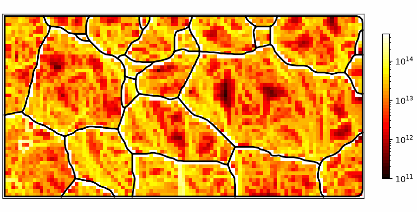
Read the map on its logarithmic scale. Bright regions require a larger energy-weighted dislocation content to reproduce the measured curvature; dark regions require less. Grain boundaries are overlaid for location, but the fitted values belong to EBSD pixels rather than boundary segments.

The maths behind the workflow

The remainder of the page expands the operations performed by calcGND. This sequence is useful when you need to inspect tensor components, change the candidate systems, or retain their individual fitted densities.

Compute the incomplete curvature tensor

The curvature tensor \(\boldsymbol\kappa\) collects directional derivatives of lattice orientation. A two-dimensional map supplies derivatives along its two in-plane directions but not along the map normal.

kappaMeasured = ebsd.curvature()
kappaMeasured

curvatureTensor (y←↑x)
  unit: 1/um
  rank: 2 (3 × 3)
  size: 101 × 51

Inspect one pixel and one component. Indexing with brackets selects map positions, counted from zero; the component \((1,2)\) over the whole map is the slice of the coefficient array M, MATLAB’s curly braces.

kappaMeasured[2, 1]

curvatureTensor (y←↑x)
  unit: 1/um
  rank: 2 (3 × 3)
  *10^-4
  -0.7842  -5.0601  NaN
  -0.5695  -5.8882  NaN
   2.0359  -1.9214  NaN

kappa12 = kappaMeasured.M[..., 0, 1]
kappa12.shape

(101, 51)

The component array has the same size as the EBSD map. For this scan the unknown out-of-plane derivative occupies the third tensor column, so that column contains NaN.

newMtexFigure(layout=[3, 3], figSize='large')
for i in range(3):
  for j in range(3):
    nextAxis(i, j)
    plot(ebsd, kappaMeasured.M[..., i, j], micronbar='off')
    hold(True)
    plot(grains.boundary, lineWidth=2)
    hold(False)
setColorRange([-0.005, 0.005])

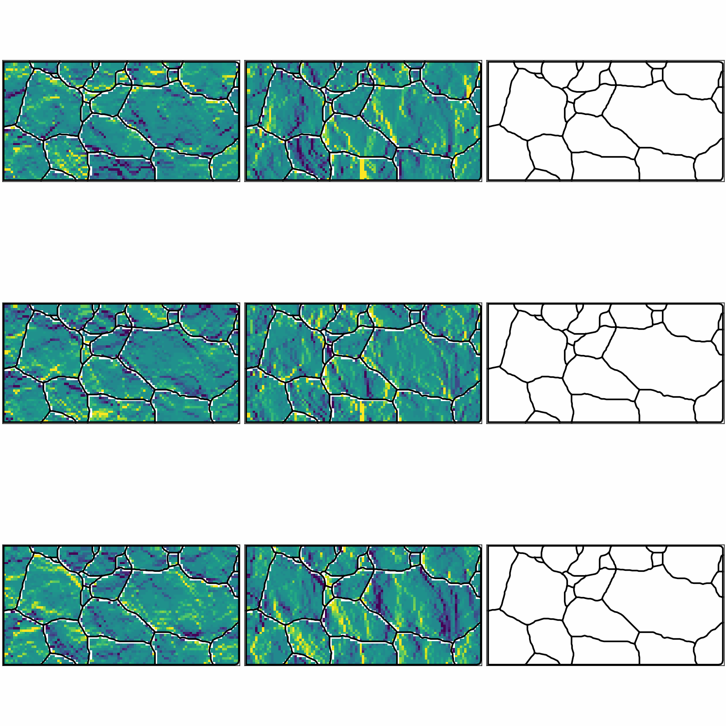
Read columns from left to right in each tensor row. The blank panels in the third column make the unmeasured out-of-plane derivative explicit; they are not zero-curvature components.

Convert curvature to the Nye tensor

Nye’s dislocation-density tensor \(\boldsymbol\alpha\) is related to curvature by

The method dislocationDensity applies this relation.

alphaMeasured = kappaMeasured.dislocationDensity()
alphaMeasured

dislocationDensityTensor (y←↑x)
  unit: 1/um
  rank: 2 (3 × 3)
  size: 101 × 51

alphaMeasured[2, 1]

dislocationDensityTensor (y←↑x)
  unit: 1/um
  rank: 2 (3 × 3)
  *10^-4
      NaN  -0.5695   2.0359
  -5.0601      NaN  -1.9214
      NaN      NaN   6.6724

This tensor remains incomplete because the map contains no derivative normal to its plane. MTEX can recover the \((3,3)\) entry from the two known diagonal curvature components, but the other missing entries remain NaN.

Rotate the candidate systems

Each tensor supplied by dS.tensor is the rank-two dyad \(\mathbf b\otimes\hat{\mathbf l}\). Its length unit is inherited from the unit cell, usually Angstrom and displayed as au.

The tensors are initially expressed in the crystal frame. The measured curvature is expressed in the specimen frame, so each pixel orientation must rotate all candidate systems into that same frame; MATLAB’s outer product ebsd.orientations * dS is a column of orientations times a row of systems.

dSRot = ebsd.orientations.reshape(-1, 1) * dS

dS[0].tensor()

dislocationDensityTensor (Iron (Alpha))
  unit: au
  rank: 2 (3 × 3)
  -1.1717  -0.5858   0.5858
   1.1717   0.5858  -0.5858
  -1.1717  -0.5858   0.5858

Fit individual system densities

fitDislocationSystems solves a linear program at every pixel. It reproduces the six measured curvature components while minimizing \(\sum_j u_j\lvert\rho_j\rvert\) over the candidate systems.

The port solves the programs with its own simplex, all pixels in parallel, where MATLAB needs the Optimization Toolbox function linprog. The result rho has one row per EBSD pixel and one column per dislocation system. Its signs distinguish the two line senses represented internally during the fit.

rhoWorked, factor = fitDislocationSystems(kappaMeasured, dSRot)
rhoWorked.shape

(5151, 52)

factor

1.0000e+16

The scale factor converts the density coefficients from \(1/(\mathrm{\mu m}\,\mathrm{au})\) to \(1/\mathrm{m}^2\). With micrometre scan units and Angstrom lattice units it is \(10^{16}\).

Reconstruct the fitted tensors

Sum each rotated basis tensor multiplied by its fitted density. The numeric matrix rhoWorked does not retain units, so the tensor unit must be restored explicitly after this manual reconstruction.

alphaFitted = (dSRot.tensor() * rhoWorked).sum(axis=1).reshape(ebsd.shape)
alphaFitted.unit = '1/um'

alphaFitted[2, 1]

dislocationDensityTensor (y←↑x)
  unit: 1/um
  rank: 2 (3 × 3)
  *10^-4
   3.7476  -0.5695   2.0359
  -5.0601  -1.3564  -1.9214
  -0.4706   -1.815   6.6724

kappaMeasured[2, 1].dislocationDensity()

dislocationDensityTensor (y←↑x)
  unit: 1/um
  rank: 2 (3 × 3)
  *10^-4
      NaN  -0.5695   2.0359
  -5.0601      NaN  -1.9214
      NaN      NaN   6.6724

The fitted tensor is complete because the chosen dislocation population supplies the components that EBSD cannot measure directly. Converting it back gives a complete fitted curvature tensor.

kappaFitted = alphaFitted.curvature()
kappaFitted

curvatureTensor (y←↑x)
  unit: 1/um
  rank: 2 (3 × 3)
  size: 101 × 51

kappaFitted[2, 1]

curvatureTensor (y←↑x)
  unit: 1/um
  rank: 2 (3 × 3)
  *10^-4
  -0.7842  -5.0601  -0.4706
  -0.5695  -5.8882   -1.815
   2.0359  -1.9214   2.1405

newMtexFigure(layout=[3, 3], figSize='large')
for i in range(3):
  for j in range(3):
    nextAxis(i, j)
    plot(ebsd, kappaFitted.M[..., i, j], micronbar='off')
    hold(True)
    plot(grains.boundary, lineWidth=2)
    hold(False)
setColorRange([-0.005, 0.005])

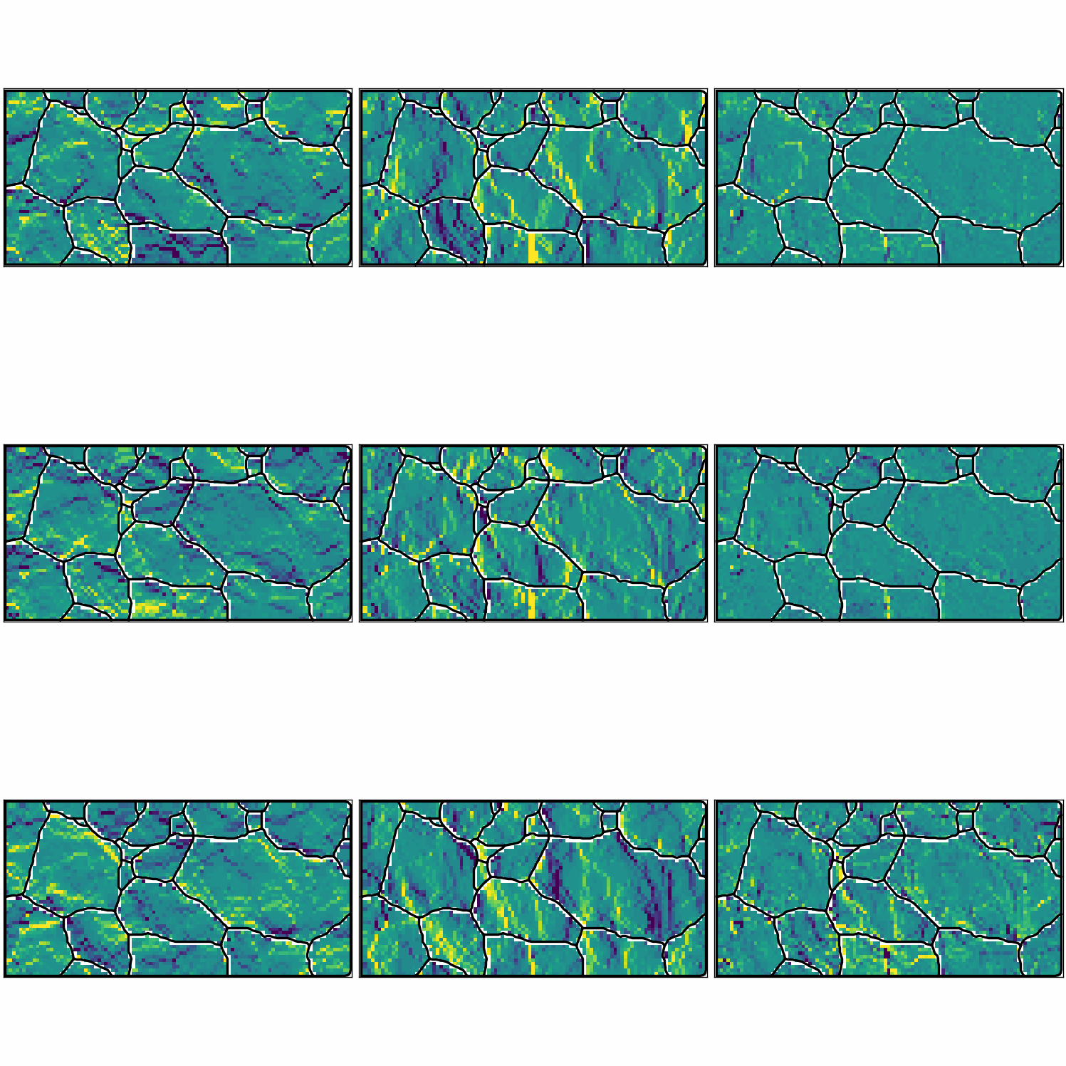
Unlike the measured grid, this grid has values in all nine panels. The fitted in-plane columns reproduce the observations; the third column is a model-dependent completion, not an additional EBSD measurement.

Reproduce the one-command result

Multiplying the absolute fitted densities by their line-energy weights and by the unit factor gives the scalar returned by calcGND.

gndWorked = factor * np.sum(np.abs(rhoWorked * dSRot.u), axis=1)
np.nanmax(np.abs(gndWorked - gnd.reshape(-1)))

0

The zero difference verifies that the expanded sequence and calcGND use the same calculation. Plotting the worked result therefore reproduces the first GND map.

plot(ebsd, gndWorked.reshape(ebsd.shape), micronbar='off')
mtexColorMap('hot')
mtexColorbar()
setColorScale('log')
setColorRange([1e11, 5e14])
hold(True)
plot(grains.boundary, lineWidth=2)
hold(False)

References

• W. Pantleon, Resolving the geometrically necessary dislocation content by conventional electron backscattering diffraction, Scripta Materialia 58 (2008), 994-997, gives the incomplete-curvature and least-energy fitting method used here.
• J. F. Nye, Some geometrical relations in dislocated crystals, Acta Metallurgica 1 (1953), 153-162, derives the dislocation-density tensor from lattice curvature.
• E. Kröner, Kontinuumstheorie der Versetzungen und Eigenspannungen, Springer, 1958, develops the continuum theory in which the curvature-dislocation relation is interpreted.
• D. Hull and D. J. Bacon, Introduction to Dislocations, fifth edition, Butterworth-Heinemann, 2011, derives the edge and screw line energies summarized on the preceding page.

Next

Continue with Weighted Burgers Vector for a boundary-based measure of lattice-curvature content that does not fit a complete population of crystallographic dislocation systems.

@article{bachmann2010mtex,
  author  = {F. Bachmann and R. Hielscher and H. Schaeben},
  title   = {Texture Analysis with MTEX - Free and Open Source Software Toolbox},
  journal = {Solid State Phenomena},
  volume  = {160},
  pages   = {63-68},
  year    = {2010},
  doi     = {10.4028/www.scientific.net/SSP.160.63},
  url     = {https://doi.org/10.4028/www.scientific.net/SSP.160.63}
}