Dislocation Systems

Plastic deformation in a crystal is carried by dislocations moving through its regular atomic lattice. A dislocation is a line defect rather than a microscopic displacement by itself.

Two vectors describe its geometry. The Burgers vector \(\mathbf b\) gives the lattice translation accumulated around the defect. The line vector \(\mathbf l\) gives the direction of the defect line.

MTEX represents a pure edge or screw geometry with a dislocationSystem. This page constructs both types and then prepares the systems used to estimate geometrically necessary dislocations from an EBSD map.

import matplotlib.pyplot as plt
import numpy as np

from mtex import *

Edge dislocations

In a pure edge dislocation, the Burgers vector is perpendicular to the line vector. Start with a cubic crystal frame and two crystal directions.

cs = crystalFrame('432')
bEdge = Miller(1, 1, 0, cs, 'uvw')
bEdge

vector3d (432)
  u  v  w
  1  1  0

lEdge = Miller(1, -1, -2, cs, 'uvw')
lEdge

vector3d (432)
  u   v   w
  1  -1  -2

The constructor checks that the two vectors are perpendicular or parallel. A general mixed dislocation cannot be entered with this constructor.

dSEdge = dislocationSystem(bEdge, lEdge)
dSEdge

dislocationSystem
  symmetry         : 432
  edge dislocations: 1
  Burgers vector  line vector  energy  length
       [1  1  0]  [1  -1  -2]       2    1.41

The grey arrow is the line vector, along which the defect runs. The red arrow is the Burgers vector, which gives the lattice shift across it.

arrow3d(1.3 * normalize(vector3d(lEdge)), faceColor=[0.45, 0.45, 0.45])
hold(True)
arrow3d(0.9 * normalize(vector3d(bEdge)), faceColor='red')
plt.axis('off')
hold(False)

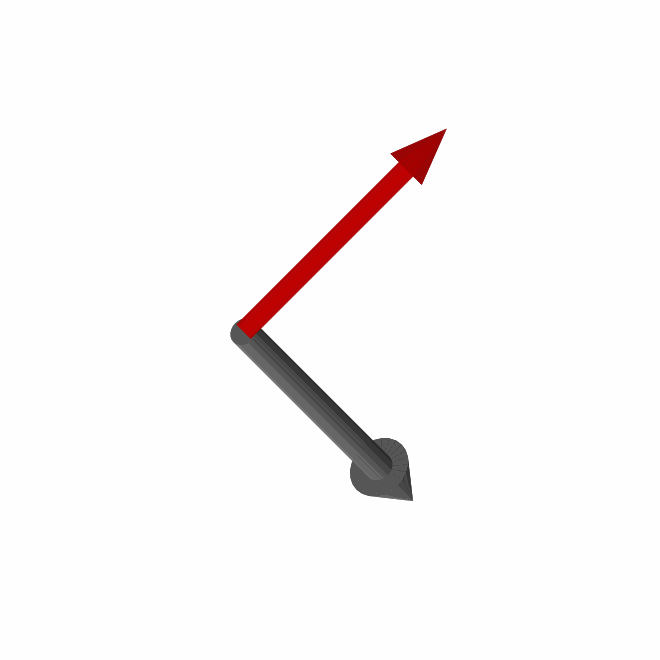
Notice that the two arrows meet at a right angle. This orthogonality is the defining geometric feature of the edge system.

Screw dislocations

In a pure screw dislocation, the Burgers vector and line vector are parallel. The same Burgers vector can therefore serve as both inputs.

bScrew = Miller(1, 1, 0, cs, 'uvw')
bScrew

vector3d (432)
  u  v  w
  1  1  0

lScrew = Miller(1, 1, 0, cs, 'uvw')
lScrew

vector3d (432)
  u  v  w
  1  1  0

dSScrew = dislocationSystem(bScrew, lScrew)
dSScrew

dislocationSystem
  symmetry          : 432
  screw dislocations: 1
  Burgers vector  energy  length
       [1  1  0]     1.4    1.41

Draw the line vector longer so that both arrows remain visible when they lie on top of one another.

arrow3d(1.3 * normalize(vector3d(lScrew)), faceColor=[0.45, 0.45, 0.45])
hold(True)
arrow3d(0.9 * normalize(vector3d(bScrew)), faceColor='red')
plt.axis('off')
hold(False)

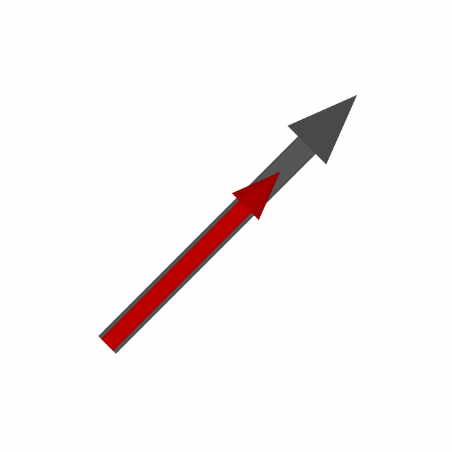
The coincident arrows show that the lattice shift is along the direction in which the defect runs. This parallelism distinguishes the screw system.

Build systems from slip systems

A slip system supplies a Burgers vector and a slip-plane normal. MTEX converts each slip system into an edge system with a line direction in the slip plane, and also adds the distinct screw systems.

Here the 12 geometrically distinct FCC slip systems produce 12 edge and 6 screw systems. The 'antipodal' option identifies opposite shear senses before the conversion.

sSFcc = symmetrise(slipSystem.fcc(cs), antipodal=True)
dSFcc = dislocationSystem(sSFcc)
[sum(dSFcc.isEdge), sum(dSFcc.isScrew)]

[12, 6]

The named constructor performs the corresponding conversion for the standard BCC family. It is a shortcut for constructing and symmetrising slipSystem.bcc(cs), not for the FCC lines above.

dSBcc = dislocationSystem.bcc(cs)
[sum(dSBcc.isEdge), sum(dSBcc.isScrew)]

[48, 4]

MTEX uses one half of the cubic slip direction as the Burgers vector during this conversion. A hexagonal slip direction is the Burgers vector itself: the direction \([11\bar{2}0]\) of MTEX has length \(a\). For other lattices the physical scale is ambiguous and the conversion is refused.

The dislocation tensor

A dislocation system contributes the dyadic tensor \(\mathbf b\otimes\hat{\mathbf l}\), where the hat denotes a unit line vector. This tensor is sometimes described informally as a deformation matrix. In MTEX it is a basis tensor for the dislocation-density tensor used on the next page.

dTBcc = dSBcc.tensor()
dTBcc

dislocationDensityTensor (432)
  unit: au
  rank: 2 (3 × 3)
  size: 52

The tensor has the same length unit as the unit-cell axes because the line vector is normalized. MTEX labels this unit au; for a lattice specified in Angstrom, its entries are therefore in Angstrom.

The Burgers-vector norm sets the scale of each basis tensor. For the unit cubic cell used here, a BCC \(\langle111\rangle/2\) Burgers vector has length \(\sqrt{3}/2\).

a = cs.aAxis.norm()
np.array([dSBcc[0].b.norm()[0], dSBcc[-1].b.norm()[0], np.sqrt(3) / 2 * a])

array([0.866, 0.866, 0.866])

The earlier statement that both BCC and FCC Burgers vectors have length \(\sqrt{3}a/2\) is not generally correct. An FCC \(\langle110\rangle/2\) Burgers vector has length \(a/\sqrt{2}\), as this check shows.

np.array([dSFcc[0].b.norm()[0], a / np.sqrt(2)])

array([0.7071, 0.7071])

Set relative line energies

The property u stores the relative line energy used when MTEX chooses a non-negative combination of systems. By default it is \(b^2\) for an edge and \(0.7\,b^2\) for a screw system, in the squared length unit of the unit cell.

Hull and Bacon give the elastic line energies

where \(G\) is the shear modulus, \(b\) is the Burgers-vector length, \(\nu\) is Poisson’s ratio, \(R\) is the outer cut-off radius, and \(r_0\) is the dislocation-core radius.

The default sets the factors all systems share to one and takes \(\nu=0.3\). Relative to the shortest Burgers vector \(b_{\min}\) the line energies are \((b/b_{\min})^2\) for an edge system and \((1-\nu)\,(b/b_{\min})^2\) for a screw system, which keeps the weights independent of the length unit and lets you choose \(\nu\).

nu = 0.3
dSBcc.u = (dSBcc.b.norm() / dSBcc.b.norm().min()) ** 2 * (1 - nu * dSBcc.isScrew)
[dSBcc.u[0], dSBcc.u[-1]]

[1.0000000000000004, 0.7]

All BCC Burgers vectors have the same length, which leaves 1 for the edge and \(1-\nu\) for the screw systems. Where families with different Burgers vectors act together the length matters: the \(\langle c+a\rangle\) systems of titanium are about 3.5 times as costly as its \(\langle a\rangle\) systems.

There is no single accepted way to set these weights. The shear modulus and the cut-off radii may differ between families, and a model may account for them. Choose u for the material and model being compared rather than treating an MTEX default as a measured energy.

References

• D. Hull and D. J. Bacon, Introduction to Dislocations, fifth edition, Butterworth-Heinemann, 2011, derives the edge and screw line energies used to motivate the relative weights above.

Next

Continue with Geometrically Necessary Dislocations to turn an EBSD orientation gradient into densities of the systems defined here.

@article{bachmann2010mtex,
  author  = {F. Bachmann and R. Hielscher and H. Schaeben},
  title   = {Texture Analysis with MTEX - Free and Open Source Software Toolbox},
  journal = {Solid State Phenomena},
  volume  = {160},
  pages   = {63-68},
  year    = {2010},
  doi     = {10.4028/www.scientific.net/SSP.160.63},
  url     = {https://doi.org/10.4028/www.scientific.net/SSP.160.63}
}