download as script · edit page

A long list of measured directions is often easier to interpret as a smooth density on the sphere. High values identify directions that occur more often than they would in a uniform population.

This page applies kernel density estimation to vector3d data. It assumes the vector construction from Defining Three-Dimensional Vectors, the direction-axis distinction from Axes and Antipodal Symmetry, and the plots introduced in Spherical Projections. The general statistical idea is developed in Density Estimation.

import matplotlib.pyplot as plt
import numpy as np

from mtex import *

plottingConvention.default('y↑→x')

From Measured Axes to a Density

The forsterite example map supplies one crystallographic c-axis for every indexed Forsterite pixel.

ebsd = mtexdata('forsterite')

cAxes = ebsd['Fo'].orientations * ebsd['Fo'].CS.cAxis
numCAxes = len(cAxes)
numCAxes

The calculation uses 152345 axes. One vector3d variable holds the entire list, which is why the object summary itself is suppressed above.

A crystallographic c-axis is an unoriented line: c and -c represent the same physical axis. The antipodal flag records that assumption.

cAxes.antipodal = True

plot(cAxes, upper=True, markerFaceColor='none', markerEdgeAlpha=0.01, markerSize=4)

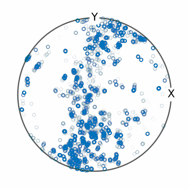
The projected sphere is almost covered by markers. Some concentrations are visible, but their relative strengths cannot be read from this overlap.

calcDensity replaces the point cloud by a continuous spherical function. Given no halfwidth, it selects one from the data, which assumes independent observations; the pixel axes of a map are not, as the section Letting the Data Choose the Halfwidth shows. So this page names MATLAB’s default, 10 degrees.

pdf = calcDensity(cAxes, halfwidth=10 * degree)
pdf

S2FunHarmonic (y↑→x)
  bandwidth: 25
  mean     : 1
  antipodal: true

The summary identifies a harmonic spherical function with bandwidth 25. It also reports antipodal: true because the estimate inherited the axis symmetry of cAxes.

plot(pdf, complete=True)
mtexColorbar()

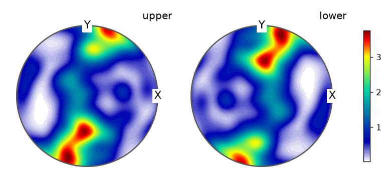
The upper- and lower-hemisphere patterns repeat through the centre of the sphere. Their unequal colour levels show the concentrations hidden by the scatter plot.

Overlaying the observations checks that the high-density regions coincide with the most crowded parts of the point cloud.

contourf(pdf)
mtexColorMap('LaboTeX')

hold(True)
plot(cAxes, upper=True, markerFaceColor='none', markerEdgeColor='k', markerEdgeAlpha=0.01, markerSize=4)
hold(False)

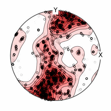
The darkest clusters of points lie inside the highest filled contours. The estimate summarizes their concentration without inventing a new location for a peak.

MTEX normalizes the density to have mean value one.

pdfMean = mean(pdf)
pdfMean

1.0000

Values are therefore multiples of uniform density (m.u.d.). A value of 3 means three times the density expected from uniformly distributed axes. It is not the fraction of axes at one exact direction; fractions require integration over a finite region.

Choosing the Halfwidth

The kernel halfwidth controls how far each observation is spread. Compare four choices on the same axes.

hw = np.array([2.5, 5, 10, 20]) * degree
mtexFig = newMtexFigure(layout=[1, 4])

for k in range(len(hw)):

  plot(calcDensity(cAxes, halfwidth=hw[k]), upper=True)
  mtexTitle(f'${hw[k] / degree:g}^{{\\circ}}$')

  if k < len(hw) - 1:
    nextAxis()

mtexFig.drawNow()

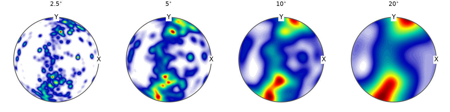
At 2.5 degrees the estimate contains many narrow peaks. At 20 degrees those peaks have merged into broad regions. A small halfwidth can preserve measurement-scale variation, while a large one can erase real structure. Neither choice is automatically more accurate.

The halfwidth also sets the harmonic bandwidth needed to represent the kernel. Print both the peak density and bandwidth for the four estimates.

for k in range(len(hw)):
  pdfK = calcDensity(cAxes, halfwidth=hw[k])
  print(f'halfwidth: {hw[k] / degree:g}° -> maximum: {max(pdfK)[0]:.2g} mud, bandwidth: {pdfK.bandwidth}')

halfwidth: 2.5° -> maximum: 14 mud, bandwidth: 92
halfwidth: 5° -> maximum: 5.7 mud, bandwidth: 48
halfwidth: 10° -> maximum: 3.8 mud, bandwidth: 25
halfwidth: 20° -> maximum: 2.5 mud, bandwidth: 13

Across this sweep the maximum falls from 14 to 2.5 m.u.d., while the bandwidth falls from 92 to 13. A sharper estimate is more expensive as well as more sensitive to fine-scale variation.

The relevant sample size is the number of independent observations, not merely the number of pixels. Neighbouring EBSD pixels are spatially correlated because many sample the same grain. calcKernel selects a halfwidth from the data with the grains taken into account; the section Letting the Data Choose the Halfwidth below applies it once the grains are reconstructed. For orientation data, ODF Estimation from EBSD Data explains this dependence and Optimal Kernel Selection describes the selection methods.

Weighting Changes the Question

A grain is a phase-homogeneous, spatially connected region of EBSD pixels produced by segmentation. Reconstruct the map with an example 10 degree misorientation threshold, then keep the Forsterite grains.

grains = calcGrains(ebsd, angle=10 * degree)
grains = grains['Fo']

# one c-axis per grain
cAxesGrains = grains.meanOrientation * grains.CS.cAxis
cAxesGrains.antipodal = True
numGrainAxes = len(cAxesGrains)
numGrainAxes

The reconstruction gives 1152 Forsterite grain axes instead of 152345 pixel axes. Giving each grain one vote describes the distribution of grains. Weighting by sectional grain area describes the mapped material area, which is the question answered by equal pixel weights on this regular scan.

mtexFig = newMtexFigure(layout=[1, 3])

plot(pdf, upper=True)
mtexTitle('one pixel - one vote')

nextAxis()
plot(calcDensity(cAxesGrains, halfwidth=10 * degree), upper=True)
mtexTitle('one grain - one vote')

nextAxis()
plot(calcDensity(cAxesGrains, weights=grains.area, halfwidth=10 * degree), upper=True)
mtexTitle('weighted by grain area')

setColorRange('equal')
mtexColorbar()
mtexFig.drawNow()

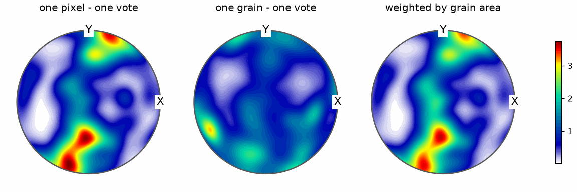
With a common colour range, equal grain weights give the flattest panel. Area weighting restores the main concentrations of the pixel estimate, although replacing every grain by its mean orientation removes the within-grain spread. The scientifically correct weights depend on whether the population of interest is grains, mapped area, or something else.

Letting the Data Choose the Halfwidth

calcKernel selects the kernel from the axes themselves; calcDensity calls it whenever no halfwidth is given. Its default method 'UCV' estimates the integrated squared error of the density for every candidate halfwidth and takes the halfwidth where the estimate is least, but never one so narrow that noise could raise bumps above a fifth of the estimate’s maximum. 'conservative' takes a halfwidth at least as wide as the optimum with high probability. Optimal Kernel Selection explains both.

Both rules take the observations as independent unless told otherwise. Pixel axes are not, and directions do not carry that knowledge, so pass the grain id of every pixel. calcGrains left the ids on ebsd. Recompute the pixel axes after reconstruction so they follow any pixels relabelled as not indexed.

rng = np.random.default_rng(0)
pixelAxes = ebsd['Fo'].orientations * ebsd['Fo'].CS.cAxis
pixelAxes.antipodal = True
pixelGrainId = ebsd['Fo'].grainId

psiAsIndependent = calcKernel(pixelAxes, 'UCV', rng=rng)
psiPixels = calcKernel(pixelAxes, 'UCV', groups=pixelGrainId, rng=rng)
psiGrainArea = calcKernel(cAxesGrains, 'UCV', weights=grains.area, rng=rng)
psiGrains = calcKernel(cAxesGrains, 'UCV', rng=rng)

for name, psi in [('pixels as independent', psiAsIndependent), ('pixels with grain ids', psiPixels),
                  ('grains weighted by area', psiGrainArea), ('grains, one vote each', psiGrains)]:
  print(f'{name:24s} {psi.halfwidth() / degree:5.3g} degree')

pixels as independent        1 degree
pixels with grain ids     21.2 degree
grains weighted by area   19.8 degree
grains, one vote each     2.46 degree

Taken as independent, the pixel axes drive the selection to the narrowest candidate, 1 degree: neighbouring pixels repeat one axis, and the rule reads the repetition as a sharp density. Even the noise floor cannot help, since with that many observations it expects hardly any noise. With the grain ids it asks for 21 degrees, close to the 20 degrees of the grain axes weighted by their area, which describe the same mapped area.

One vote per grain asks for 2.5 degrees, the narrowest kernel the noise floor admits for 1152 axes. Many grains are single pixels, mostly fragments beside a grain of nearly the same orientation, so the grain axes repeat each other as well. The area weight gives those fragments almost no say.

The conservative rule on the pixels with their grain ids:

psiConservative = calcKernel(pixelAxes, 'conservative', groups=pixelGrainId, rng=rng)
psiConservative.halfwidth() / degree

24.3419

It asks for 24 degrees, a little wider than UCV’s 21, as it should: it takes the energies of the axis distribution at their lower confidence bounds. Weighted by area, the few large grains dominate the map, which leaves these bounds loose. A reported halfwidth is worth checking against the plots of the previous section rather than taken on trust.

Working with the Density Function

A density is an S2Fun, so it can be evaluated, integrated, searched for peaks, combined with other spherical functions, and sampled. Operations on Spherical Functions develops that common interface.

First find the global maximum.

globalDensity, globalPos = max(pdf)
globalDensity

3.7532

globalPos

vector3d (y↑→x)
  antipodal: true
       x       y      z
  -0.295  -0.941  0.165

The output gives both the density and the specimen direction where it is attained. The numLocal option requests several distinct local maxima.

localDensity, localPos = max(pdf, numLocal=3)
localDensity

array([3.7532, 3.7026, 2.9869])

localPos

vector3d (y↑→x)
  size     : 3
  antipodal: true
        x       y      z
   -0.295  -0.941  0.165
  -0.0541  -0.668  0.742
    0.114   0.833  0.542

The first local maximum is the global one. Integrate the density within 20 degrees of that axis using volume.

smoothedFraction = volume(pdf, localPos[0], 20 * degree)
smoothedFraction

0.1721

The smoothed estimate assigns 0.1723, or 17.23 percent, of the population to that axial neighbourhood. Count the original axes in the same region.

observedFraction = np.mean(angle(cAxes, localPos[0]) < 20 * degree)
observedFraction

0.1890

The direct count is 0.1890, or 18.90 percent. Smoothing moves some density across the boundary of the 20 degree neighbourhood, so the two questions do not have to give the same answer.

Evaluate the density at the three specimen basis directions.

basisDensities = pdf.eval(cat(vector3d.X, vector3d.Y, vector3d.Z))
basisDensities

array([0.458 , 1.6142, 1.2212])

Among X, Y and Z, the Y direction has the largest density in this example. If only these values are needed, pass the evaluation directions directly:

f = calcDensity(cAxes, cat(vector3d.X, vector3d.Y, vector3d.Z))

A random sample from the estimate can replace the large point cloud in a simulation or exploratory plot.

vRand = discreteSample(pdf, 500)

plot(pdf, upper=True)
hold(True)
plot(vRand, markerFaceColor='k', markerSize=4)
hold(False)

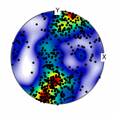
The 500 black points follow the same broad concentrations as the coloured density, but retain the sampling variation expected from a finite draw. They are simulated representatives, not a lossless compression of the original 152345 measurements.

Crystal Directions and Symmetry

The previous density lives in the specimen reference frame. An inverse pole density instead fixes a specimen direction and asks which crystal directions are parallel to it. Express specimen Z in the crystal frame of every Forsterite orientation.

h = inv(ebsd['Fo'].orientations) * vector3d.Z

The result is a list of crystal directions carrying the Forsterite crystal symmetry. calcDensity transfers that symmetry to the density automatically.

ipdf = calcDensity(h, halfwidth=10 * degree)
ipdf

S2FunHarmonic (Forsterite)
  bandwidth: 25
  mean     : 1
  antipodal: true

The summary identifies an antipodal harmonic function with the Forsterite frame. Plotting only the fundamental sector shows every symmetry-inequivalent crystal direction once.

plot(ipdf, contourf=True)
mtexColorbar()

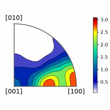
The coloured sector contains the complete inverse pole density without repeating symmetry-related directions. The symmetry=False option disables crystal symmetrization when that is deliberately required.

Choosing a Different Kernel

The default is the non-negative de la Vallee Poussin kernel. Its finite harmonic expansion avoids truncation ringing. The kernel option also accepts other spherical kernels.

Compare the default 10 degree kernel with a Dirichlet kernel truncated at bandwidth 12.

psi1 = S2DeLaValleePoussinKernel(halfwidth=10 * degree)
psi2 = S2DirichletKernel(12)

plot(psi1, lineWidth=2)
hold(True)
plot(psi2, lineWidth=2)
hold(False)
plt.xlim(0, 60)
plt.legend(['de la Vallee Poussin', 'Dirichlet'])

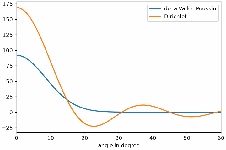
The de la Vallee Poussin curve decreases without crossing zero. The Dirichlet curve oscillates above and below zero, and those negative lobes pass into a density estimate made with it.

pdf2 = calcDensity(cAxes, kernel=psi2)

plot(pdf2, upper=True)
mtexColorbar()

minimumDirichletDensity = min(pdf2)[0]
minimumDirichletDensity

-0.4029

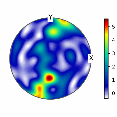
The minimum is -0.4029, which is not a valid probability density. Non-negative kernels are therefore the appropriate default for density estimation. A Dirichlet kernel remains useful for operations where exact harmonic truncation, rather than non-negativity, is the objective.

Density Estimation While Plotting

Smooth plotting options for a large vector3d list perform density estimation internally. The contourf, smooth and pcolor modes use a 5 degree halfwidth when none is supplied.

plot(cAxes, contourf=True, upper=True)
mtexColorMap('LaboTeX')
mtexColorbar()

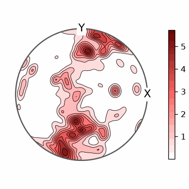
This 5 degree plot is sharper than the explicit 10 degree estimate pdf. Use calcDensity explicitly when the density itself, its weights, its kernel, or a reproducible smoothing choice matters.

The Maths Behind the Estimate

Let \(v_n\) be unit directions with non-negative weights \(w_n\), and let \(\psi\) be a normalized radial kernel. MTEX computes the weighted kernel estimate

\[f(v) = \frac{1}{\sum_{n=1}^{N}w_n} \sum_{n=1}^{N} w_n\,\psi(v\mathbin{\cdot}v_n).\]

Equal weights reduce the denominator to \(N\). For axial input, the result is symmetrized so that \(f(v)=f(-v)\). The normalization makes the mean of \(f\) equal to one under MTEX’s uniform spherical measure.

The estimate is a model of an unknown population density, not the unknown density itself. Decreasing the halfwidth reduces smoothing bias but raises sampling variation; increasing it does the reverse.

Spherical Density Estimation