This script demonstrates a systematic approach on how to get the most out of challenging PGR tasks by systematic tuning of the most critical parameters. The microstructure explored in this example is lath martensite, for which especially the reconstruction of annealing twins in the parent austenite phase is a challenging task. This is the same dataset that is explored in the general documentation for martensite Parent Grain Reconstruction.
As the script is quite long and some sections take some time to execute, I highly recommend running this script section-by-section. You ideally want to follow my talk at the MTEX User Meeting 2024 before or alongside exploring this script.
Data Import
Let us begin by loading the MTEX documentation dataset on martensite from Ref. T. Nyyssönen, P. Peura, V.-T. Kuokkala, Crystallography, Morphology, and Martensite Transformation of Prior Austenite in Intercritically Annealed High-Aluminum Steel, Metall Mater Trans A 49 (2018) 6426–6441.
% get MTEX data
mtexdata martensite silent

% set plotting convention
setMTEXpref('xAxisDirection','east');
setMTEXpref('zAxisDirection','outofPlane');
Plot the EBSD data of the child phase
Let us first take a look at the example EBSD data.
% Define color key
ipfKey = ipfColorKey(ebsd);
ipfKey.inversePoleFigureDirection = vector3d.Z;

% Get colors associated with crystal orientations
colors = ipfKey.orientation2color(ebsd.orientations);

% Plot the microstructure data
figure('Name','Martensitic microstructure')
plot(ebsd,colors);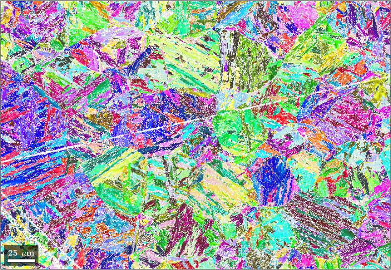
We can see that the dataset only consists of lath martensite, the child phase in this transformation system, and unindexed points. Our aim is to accurately reconstruct the prior austenite microstructure, the parent microstructure in this example.
Explore different threshold angles for child grain reconstruction
Let us explore some different threshold angles to reconstruct the child grains at different levels of detail.
%List of threshold angles
thrsh_angles = [6,3,2,1.5,1];

%Prepare plotting
figure;
f(1) = newMtexFigure('layout',[2,3],'Name','Child grain reconstruction at different threshold angles');

% Loop over different child grain reconstructions
for ii = 1:length(thrsh_angles)

  % Load data
  mtexdata martensite silent

  % Calculate grains with defined angular threshold
  [grains,ebsd.grainId] = calcGrains(ebsd('indexed'), 'angle',thrsh_angles(ii)*degree);
  ebsd(grains(grains.grainSize < 3)) = [];
  [grains,ebsd.grainId] = calcGrains(ebsd('indexed'),'angle',thrsh_angles(ii)*degree);
  grains = smooth(grains,5);

  % Plot the orientation data and overlay the grain boundaries
  plot(ebsd,ebsd.orientations);
  hold on
  plot(grains.boundary)
  title(strcat("Threshold angle: ", num2str(thrsh_angles(ii),"%.1f"), "^{\circ}"),...
    'interpreter','tex');
  hold off

  % Enable multiplot
  if ii < length(thrsh_angles), nextAxis; end
end
From the child grain reconstructions it is apparent that in this dataset threshold values of 1 to 1.5° lead to a significant loss of EBSD data associated with small grains. Therefore only the range of 2-6° is feasible as a starting point for grain reconstruction.
Effect of child grain reconstruction on PGR results
We will now carry out the PGR on child grains reconstructed with the identified angular threshold values. We will otherwise assume reasonable and constant parameters for the PGR to enable comparability. We compare the PGR results as received from the variant graph approach before any post-processing to enable reasonable comparison
% Let us revisit the three largest threshold angles
thrsh_angles = thrsh_angles(1:3);

%Prepare plotting
figure;
f(2) = newMtexFigure('layout',[1,length(thrsh_angles)],'Name','PGR at different Child grain threshold values');

%Child grain reconstruction
for ii = 1:length(thrsh_angles)

  % Load data
  mtexdata martensite silent

  % Calculate grains with defined angular threshold
  [grains,ebsd.grainId] = calcGrains(ebsd('indexed'), 'angle',thrsh_angles(ii)*degree);
  ebsd(grains(grains.grainSize < 3)) = [];
  [grains,ebsd.grainId] = calcGrains(ebsd('indexed'),'angle',thrsh_angles(ii)*degree);
  grains = smooth(grains,5);

  % set up the PGR job
  job = parentGrainReconstructor(ebsd,grains);

  % initial guess for the parent to child orientation relationship
  job.p2c = orientation.KurdjumovSachs(job.csParent, job.csChild);

  % refine the OR
  job.calcParent2Child;

  % setup the variant graph
  job.calcVariantGraph('threshold',2.5*degree,'tolerance',2.5*degree);

  % cluster the variant graph
  job.clusterVariantGraph;

  % calculate the parent grain orientations
  job.calcParentFromVote('minProb',0.5);

  % plot the parent grains (before any further processing)
  plot(job.parentGrains,job.parentGrains.meanOrientation)
  title(strcat("Threshold angle: ", num2str(thrsh_angles(ii),"%.1f"), "^{\circ}"),...
    'interpreter','tex');

  % Enable multiplot
  if ii < length(thrsh_angles), nextAxis; end
end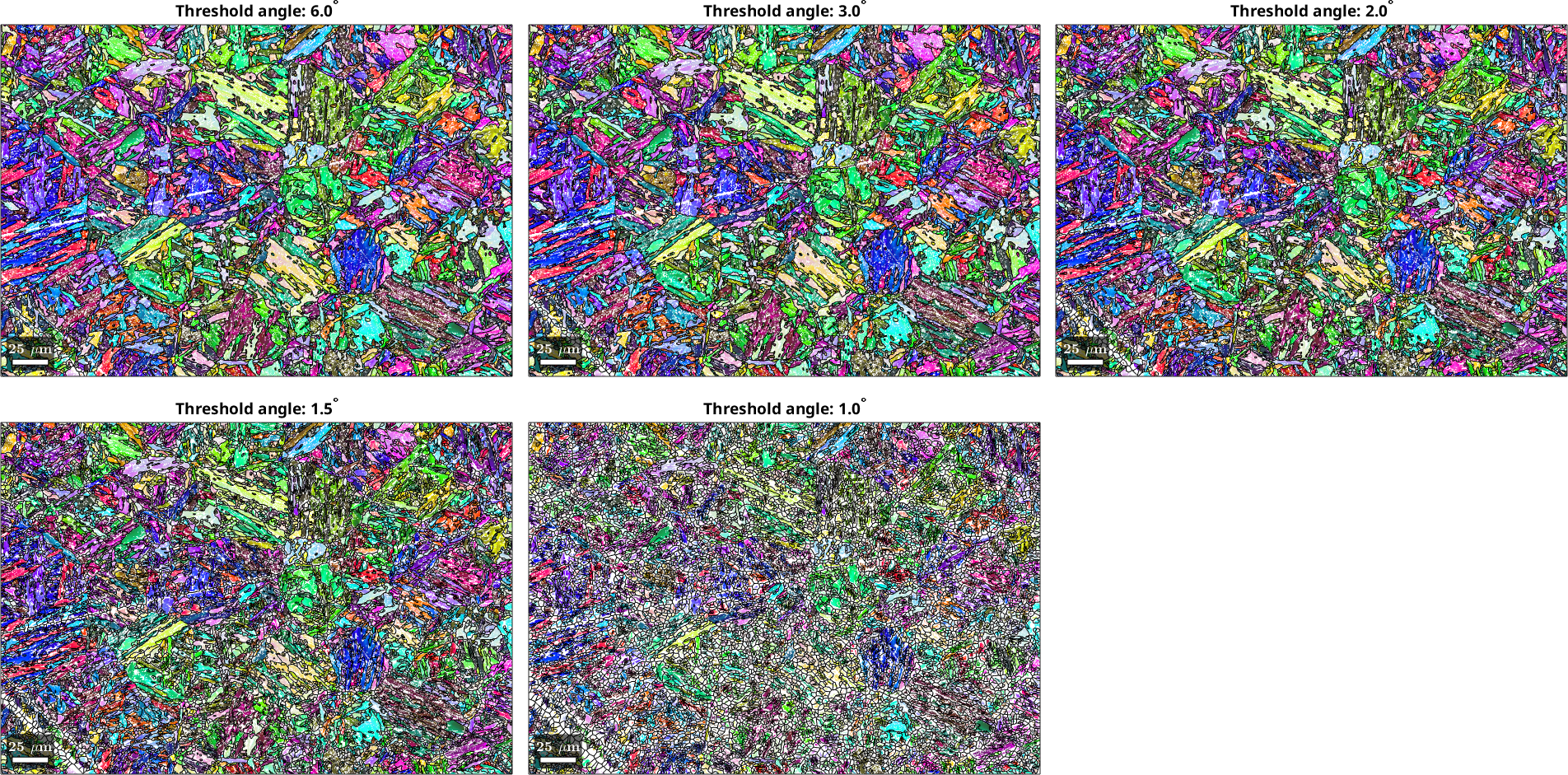
The effect of child grain reconstruction appears to be quite prominent - the smaller the reconstruction threshold angle the more of the parent grain microstructure is confidently reconstructed. In martensitic steels the misorientation between the different variants is oftentimes quite low which means that grain reconstruction with too large threshold values merges grains that belong to different variants and thereby complicate the PGR. For this example, 2° seems to be the optimum, so we will move forward with that parameter.
Optimizing the orientation relationship (OR)
Next we will check the effect of fitting the OR using the calcParent2Child function vs. assuming several rational ORs on PGR.
% Load data
mtexdata martensite silent

% Calculate grains with defined angular threshold
[grains,ebsd.grainId] = calcGrains(ebsd('indexed'), 'angle',2*degree);
ebsd(grains(grains.grainSize < 3)) = [];
[grains,ebsd.grainId] = calcGrains(ebsd('indexed'),'angle',2*degree);
grains = smooth(grains,5);

% Initialize the parent grain reconstructor class
job = parentGrainReconstructor(ebsd,grains);

% Define some rational ORs typical for lath martensitic steels
KS = orientation.KurdjumovSachs(job.csParent,job.csChild);
NW = orientation.NishiyamaWassermann(job.csParent,job.csChild);
GT = orientation.GreningerTrojano(job.csParent,job.csChild);

% initial guess for the parent to child orientation relationship
job.p2c = KS;

% iteratively refine the OR
job.calcParent2Child;

% collect all ORs (|job.p2c| contains the refined OR)
ORs = [KS,NW,GT,job.p2c];
ORnames = ["KS","NW","GT","Fitted"];

% Show the disorientation between the ORs and the misorientations at the
% microstructure grain boundaries

%Prepare plotting
figure;
f(3) = newMtexFigure('layout',[2,2],'Name','OR-Fit grain boundary plot');
fh = figure('Name','OR-Fit histogram');

% loop over different ORs
for ii = 1:length(ORs)
  %Assign OR as currently active OR
  job.p2c = ORs(ii);

  % compute the misfit for all child to child grain neighbours
  [fit,c2cPairs] = job.calcGBFit;

  % Plot the misfit in histogram
  figure(fh);
  hold on
  histogram(fit./degree,'BinMethod','sqrt');
  xlabel('Misfit Angle (^{\circ})',"Interpreter","tex");
  ylabel('Counts');
  hold off

  % select grain boundary segments by grain ids
  [gB,pairId] = job.grains.boundary.selectByGrainId(c2cPairs);

  % plot the child phase
  figure(f(3).parent);
  plot(ebsd,ebsd.orientations,'faceAlpha',0.5)

  % and on top of it the boundaries colorized by the misfit
  hold on;
  % scale fit between 0 and 1 - required for edgeAlpha
  plot(gB, 'edgeAlpha', (fit(pairId) ./ degree - 2.5)./2 ,'linewidth',2);
  hold off
  title(ORnames(ii));

  % Enable multiplot
  if ii < length(ORs), figure(f(3).parent); nextAxis; end
end

% Adding labels and titles
figure(fh);
grid on
legend(ORnames);
Warning: grains.grainSize is depreciated. Please use
grains.numPixel instead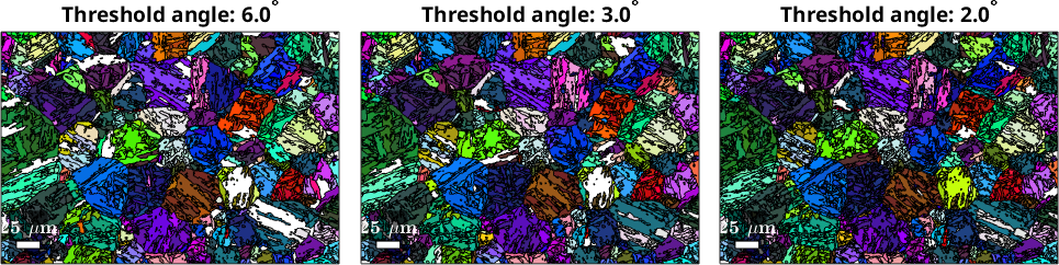
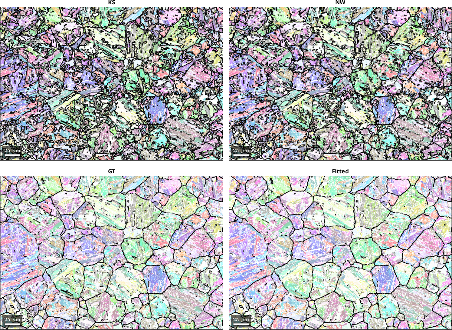
The histogram plot shows that OR refinement yields an OR that is far more representative of the actual OR present in the microstructure. The Greninger-Trojano (GT) OR is closest to the fitted OR. Plotting the fit of the OR onto the grain boundaries showed that the fitted OR nicely outlines the grain boundaries of the parent grains, which is an important prerequisite for successful PGR.
Tune parameters for OR refinement
The OR refinement using calcParent2Child can be fine-tuned with custom choices for the parameters threshold and quantile. The threshold value is the maximum misfit between the OR and grain misorientations to be considered for the optimization of the OR. The quantile value defines which quantile of the misfit distribution (see previous histogram) is considered for optimization of the OR. Whichever criterion cuts off more of the available data will be enforced. The parameters are used to make sure that the parent grain boundaries, which are not OR-related boundaries, can be excluded from the OR refinement procedure in a controlled manner.
% Let us define some parameters
% (you may want to explore more parameter sets)
threshold = [10,10,5,5];
quantile = [0.9,0.8,0.9,0.8];
% Prepare plotting
figure;
f(4) = newMtexFigure('layout',[2,2],'Name','OR-Fit grain boundary plot');
fh2 = figure('Name','OR-Fit histogram');
% loop over different parameter sets
for ii = 1:length(threshold)
%Assign initial guess for OR
job.p2c = KS;
% Refine OR
job.calcParent2Child('quantile',quantile(ii),'threshold',threshold(ii)*degree);
% Compute the misfit for all child to child grain neighbours
[fit,c2cPairs] = job.calcGBFit;
% Plot misfit distribution in histogram
figure(fh2);
hold on
histogram(fit./degree,'BinMethod','sqrt','facealpha',0.3);
xlabel('Misfit Angle (^{\circ})',"Interpreter","tex");
ylabel('Counts');
hold off
% Select grain boundary segments by grain ids
[gB,pairId] = job.grains.boundary.selectByGrainId(c2cPairs);
% Plot the child phase
figure(f(4).parent);
plot(ebsd,ebsd.orientations,'faceAlpha',0.5)
% and on top of it the boundaries colorized by the misfit
hold on;
% Scale fit between 0 and 1 - required for edgeAlpha
plot(gB, 'edgeAlpha', (fit(pairId) ./ degree - 2.5)./2 ,'linewidth',2);
hold off
title(strcat("Threshold: ",num2str(threshold(ii))," Quantile: ", num2str(quantile(ii))));
% Enable multiplot
if ii < length(threshold)
figure(f(4).parent); nextAxis;
end
end
% Adding labels
figure(fh2);
grid on
xlim([0,10])
legend(append("Thresh.: ",string(threshold),", Quantile: ",string(quantile)));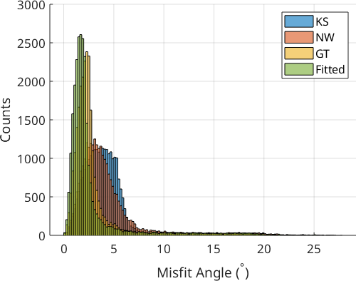
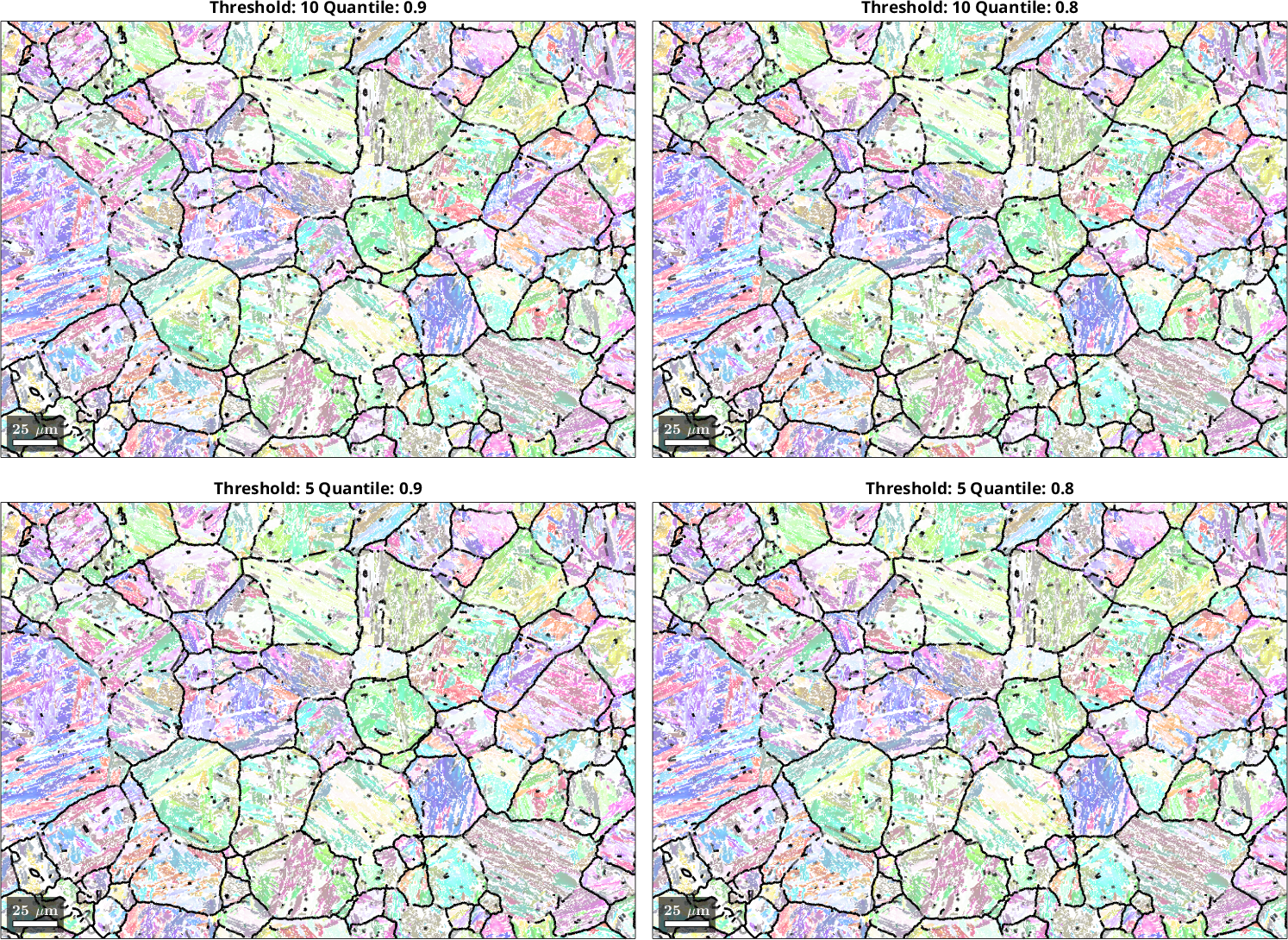
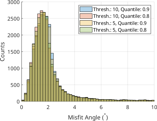
We only look at the 0° - 10° misfit range to better discern the effect of the different parameter sets. The parameter choice of the calcParent2Child command did not cause drastic changes in the fit of the optimal OR. Threshold values of 10° gave a better fit than 5°, and a quantile value of 0.9 may be slightly better than 0.8. The threshold angle of 10° and the quantile of 0.9 are the default values of the calcParent2Child command. For your dataset, the quantile value should reflect the ratio between prior parent boundaries and OR-related boundaries. In the present case, prior austenite grains are large and filled with a very fine OR-related boundary structure within, meaning that the quantile value does not play a big role. If you have small prior parent grains with little internal OR-related boundary structure you should explore smaller quantile values.
Translating the OR misfit into a probability function
Next, we need to translate the misfit between the OR and the grain misorientations \(\omega\) into an OR probability function \(\Psi\):
\begin{equation} \Psi(\omega) = 1 - \tfrac{1}{2}\left(1 + \mathrm{erf}(2 \tfrac{\omega - \delta}{\sigma})\right). \end{equation}
where \(\delta\) is a threshold value and \(\sigma\) is a tolerance value. The function tends to 1 for grain misorientations that agree well with the OR and to 0 for child grain misorientations that disagree strongly with the OR. The function therefore describes the probability with which two grains belong to the same parent grain. Let us plot this probability function on top of the OR misift distribution from before for few different combinations of the parameters tolerance and threshold.
% Let u assume an OR and iteratively refine it.
job.p2c = KS;
job.calcParent2Child;
% Plot the misfit histogram
% (|pdf| normalization was chosen to plot the misfit distribution and
% probability function with reference to the same y-axis)
figure('Name','OR-probability functions')
hold on
h = histogram(fit./degree,'BinMethod','sqrt','normalization','pdf',...
'FaceAlpha',0.3,'DisplayName',"OR misfit distribution");
% Parameter sets for tolerance and threshold
tol = [2.5,1.5,1.5,2.0];
threshold = [2.5,3.5,1.5,5.0];
% Define xLim and input vector for function
maxX = 6;
x = 0:0.1:maxX;
% Add the probability functions to the plot
hold on
xlabel('Misfit Angle (^{\circ})',"Interpreter","tex");
ylabel('Probability');
% Compute the CDF values for the normal distribution
for ii = 1:length(tol)
y = 1 - 0.5 * (1 + erf(2*(x - threshold(ii))./tol(ii)));
hold on
plot(x, y, 'LineWidth', 2, 'DisplayName',...
strcat('Tol: ',num2str(tol(ii)), "^{\circ}, Thresh: ", ...
num2str(threshold(ii)),"^{\circ}"));
end
% Format plot and figure
grid on;
legend("Interpreter","tex");
xlim([0,maxX])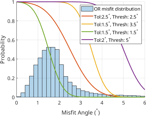
It can be observed that the different parameter choices for threshold and tolerance give a different weighting to the misfit values. Let us now plot the function values directly onto the grain boundaries to decide which parameter set leads to the best separation of prior parent and OR-related boundaries.
% compute the misfit for all child to child grain neighbors
[fit,c2cPairs] = job.calcGBFit;
% select grain boundary segments by grain ids
[gB,pairId] = job.grains.boundary.selectByGrainId(c2cPairs);
%Prepare plotting
figure;
f(5) = newMtexFigure('layout',[2,2],'Name','OR-probability grain boundary plot');
%Loop over probability function parameters
for ii = 1:length(tol)
% plot the child phase
plot(ebsd,ebsd.orientations,'faceAlpha',0.5)
% and on top of it the boundaries colorized by the misfit
hold on;
% scale fit between 0 and 1 with different parameter sets
plot(gB, 'edgeAlpha', (fit(pairId) ./ degree - threshold(ii))./tol(ii) ,'linewidth',2);
hold off
title(strcat('Tol: ',num2str(tol(ii)), "^{\circ}, Thresh: ", ...
num2str(threshold(ii)),"^{\circ}"),"Interpreter","tex");
% Enable multiplot
if ii < length(tol)
figure(f(5).parent); nextAxis;
end
end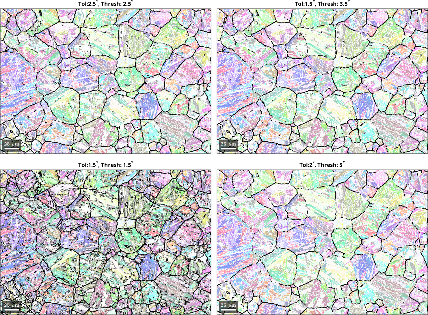
We can see that a sharp tolerance of 1.5° and threshold value of 1.5° mark several boundaries as prior austenite boundaries, even though they are in the interior of what appears to be the prior austenite grains. Conversely, a very relaxed value pair of tolerance 2° and threshold 5° does not highlight boundaries that appear to be prior austenite boundaries. The value pair tolerance 2.5° and threshold 2.5° seems to deliver the best result. In the misfit distribution histogram, this parameter set nicely separates the mode of the distribution from the tail to the right. You will have to experiment with these parameters for your own microstructure to get the best possible PGR result.
Evaluating effect of probability functions on PGR
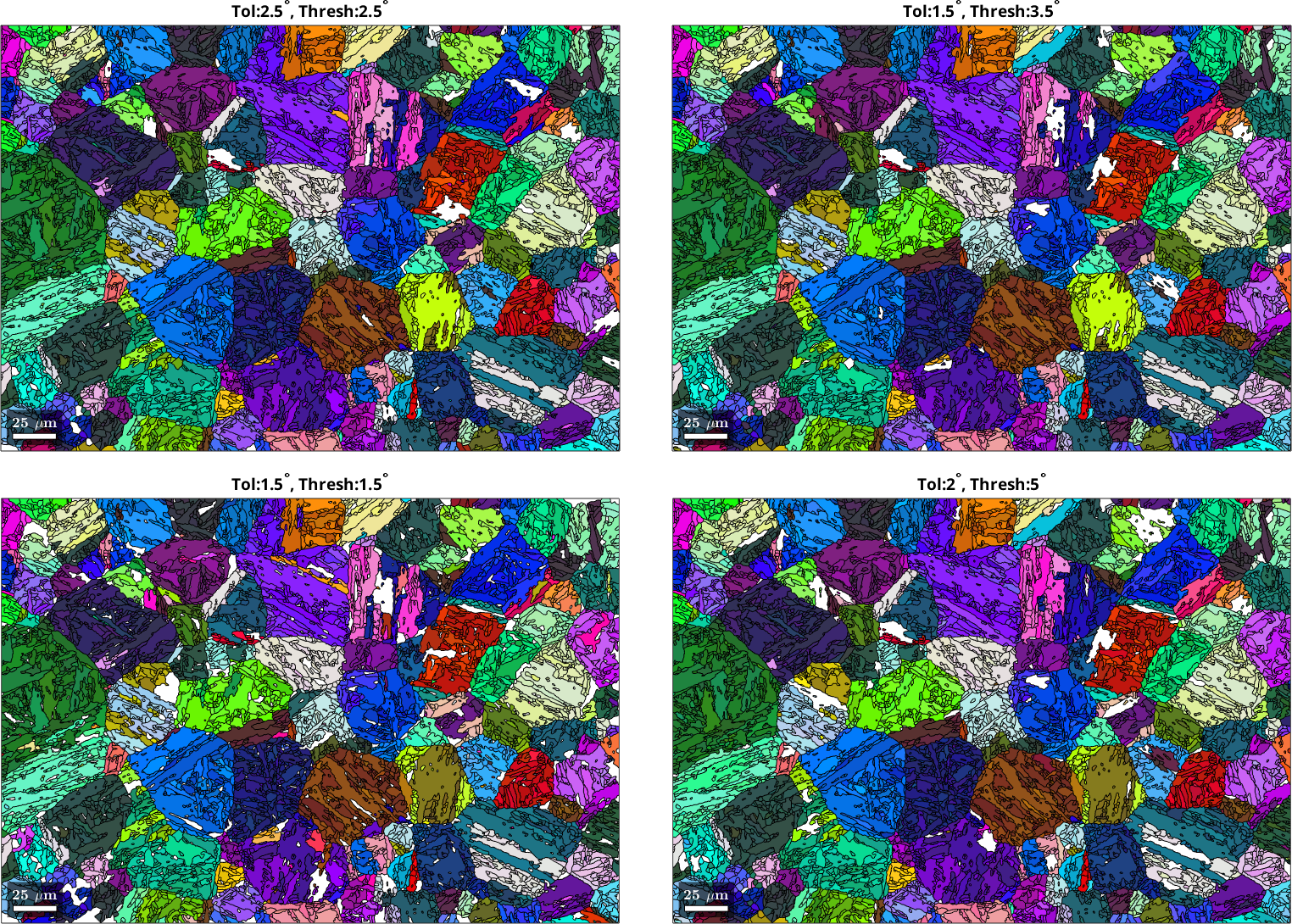
Let us now explore the PGR results that are obtained using the different probability function values. The parameters defining the probability function are passed to the method calcVariantGraph. This method sets up the variant graph, in which all possible parent variants of each grain are represented as nodes. The parent variants of neighboring grains are connected with edges that contain the computed OR probability values.
%Prepare plotting
figure;
f(6) = newMtexFigure('layout',[2,2],'Name','PGR results for different OR-probability functions');
%Loop over probability function parameters
for ii = 1:length(tol)
% setup the variant graph
job.calcVariantGraph('threshold',threshold(ii).*degree,...
'tolerance',tol(ii)*degree);
% cluster the variant graph
job.clusterVariantGraph;
% calculate the parent grain orientations
job.calcParentFromVote('minProb',0.5);
% Plot the PGR result (before any cleaning is applied)
plot(job.parentGrains,job.parentGrains.meanOrientation);
title(strcat('Tol: ',num2str(tol(ii)), "^{\circ}, Thresh:", ...
num2str(threshold(ii)),"^{\circ}"),"Interpreter","tex");
% Enable multiplot
if ii < length(tol)
figure(f(6).parent); nextAxis;
end
% Revert PGR results to allow new PGR with different parameters
job.revert;
endWarning: grains.grainSize is depreciated. Please use
grains.numPixel instead
Warning: grains.grainSize is depreciated. Please use
grains.numPixel instead
Warning: grains.grainSize is depreciated. Please use
grains.numPixel instead
Warning: grains.grainSize is depreciated. Please use
grains.numPixel instead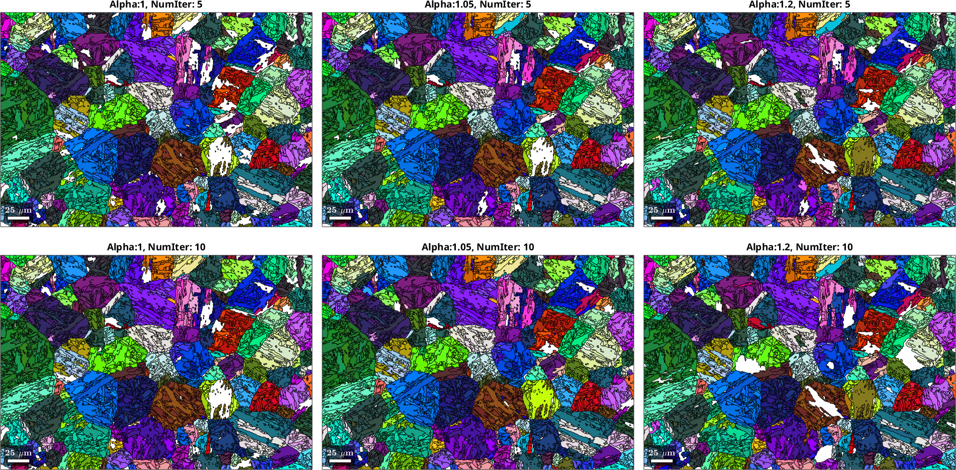
We can observe that in the case where the probability function did not lead to a good separation between prior-parent and OR-related boundaries fewer grains have been confidently reconstructed. The first two explored parameter sets give decent PGR result, with the first dataset (subjectively) looking slightly more complete. The difference here is however marginal. It is important to make this evaluation before any post-processing is applied to the reconstructed parent microstructure.
The effect of clustering parameters on the PGR
Having identified an optimal probability function to translate the OR misfit into OR probabilities, the parameters during clustering can be explored. The variant graph relies on a Markovian clustering algorithm, which is originally reported in
and defined in the present application in
When iteratively applying the Markovian clustering algorithm to the variant graph, edges with high probability are further strengthened and edges with low probability are further weakened, leading to eventual cluster formation. With each iteration the probabilities are extended to an additional order of neighbors, leading to a gradual delocalization of the optimal parent grain orientation solution.
We will explore the two most critical parameters controlling the behavior of the Markovian Clustering algorithm, numIter and inflationPower. The parameter numIter controls the number of iterations for which the clustering algorithm is run, which affects the order of neighbors taken into account and to which degree convergence is approached. The parameter inflationPower, controls the degree of clustering in each iteration. In other words, it decides how rapidly clusters are formed.
% Different settings for inflationPower (alpha) and numIter for
% MCL clustering
alpha = [1,1.05,1.2,1,1.05,1.2];
numIter = [5,5,5,10,10,10];
%Prepare plotting
figure;
f(7) = newMtexFigure('layout',[2,3],'Name','PGR results for different clustering parameters');
% Check reconstructed microstructure for different clustering parameters
for ii = 1:length(alpha)
% setup the variant graph
job.calcVariantGraph('threshold',2.5*degree,'tolerance',2.5*degree)
% cluster the variant graph with different parameters
job.clusterVariantGraph('inflationPower',alpha(ii),'numIter',numIter(ii));
% calculate the parent grain orientations
job.calcParentFromVote('minProb',0.5);
% Plot the PGR result (before any cleaning is applied)
plot(job.parentGrains,job.parentGrains.meanOrientation);
title(strcat('Alpha: ',num2str(alpha(ii)), ", NumIter: ", num2str(numIter(ii))));
% Enable multiplot
if ii < length(alpha)
figure(f(7).parent); nextAxis;
end
% Revert PGR results to allow new PGR with different parameters
job.revert;
endans = parentGrainReconstructor
phase mineral symmetry grains area reconstructed
parent Iron fcc 432 0 0% 0%
child Iron bcc (old) 432 9338 100%
OR: (347.2°,9°,56.8°)
c2c fit: 1.2°, 1.6°, 2°, 2.7° (quintiles)
closest ideal OR: (111) || (011) [1-10] || [100] fit: 2.4°
variant graph: 438720 entries
Warning: grains.grainSize is depreciated. Please use
grains.numPixel instead
ans = parentGrainReconstructor
phase mineral symmetry grains area reconstructed
parent Iron fcc 432 0 0% 0%
child Iron bcc (old) 432 9338 100%
OR: (347.2°,9°,56.8°)
c2c fit: 1.2°, 1.6°, 2°, 2.9° (quintiles)
closest ideal OR: (111) || (011) [1-10] || [100] fit: 2.4°
variant graph: 438720 entries
Warning: grains.grainSize is depreciated. Please use
grains.numPixel instead
ans = parentGrainReconstructor
phase mineral symmetry grains area reconstructed
parent Iron fcc 432 0 0% 0%
child Iron bcc (old) 432 9338 100%
OR: (347.2°,9°,56.8°)
c2c fit: 1.2°, 1.6°, 2°, 2.7° (quintiles)
closest ideal OR: (111) || (011) [1-10] || [100] fit: 2.4°
variant graph: 438720 entries
Warning: grains.grainSize is depreciated. Please use
grains.numPixel instead
ans = parentGrainReconstructor
phase mineral symmetry grains area reconstructed
parent Iron fcc 432 0 0% 0%
child Iron bcc (old) 432 9338 100%
OR: (347.2°,9°,56.8°)
c2c fit: 1.2°, 1.6°, 2°, 2.8° (quintiles)
closest ideal OR: (111) || (011) [1-10] || [100] fit: 2.4°
variant graph: 438720 entries
Warning: grains.grainSize is depreciated. Please use
grains.numPixel instead
ans = parentGrainReconstructor
phase mineral symmetry grains area reconstructed
parent Iron fcc 432 0 0% 0%
child Iron bcc (old) 432 9338 100%
OR: (347.2°,9°,56.8°)
c2c fit: 1.2°, 1.6°, 2°, 2.7° (quintiles)
closest ideal OR: (111) || (011) [1-10] || [100] fit: 2.4°
variant graph: 438720 entries
Warning: grains.grainSize is depreciated. Please use
grains.numPixel instead
ans = parentGrainReconstructor
phase mineral symmetry grains area reconstructed
parent Iron fcc 432 0 0% 0%
child Iron bcc (old) 432 9338 100%
OR: (347.2°,9°,56.8°)
c2c fit: 1.2°, 1.6°, 2°, 2.8° (quintiles)
closest ideal OR: (111) || (011) [1-10] || [100] fit: 2.4°
variant graph: 438720 entries
Warning: grains.grainSize is depreciated. Please use
grains.numPixel instead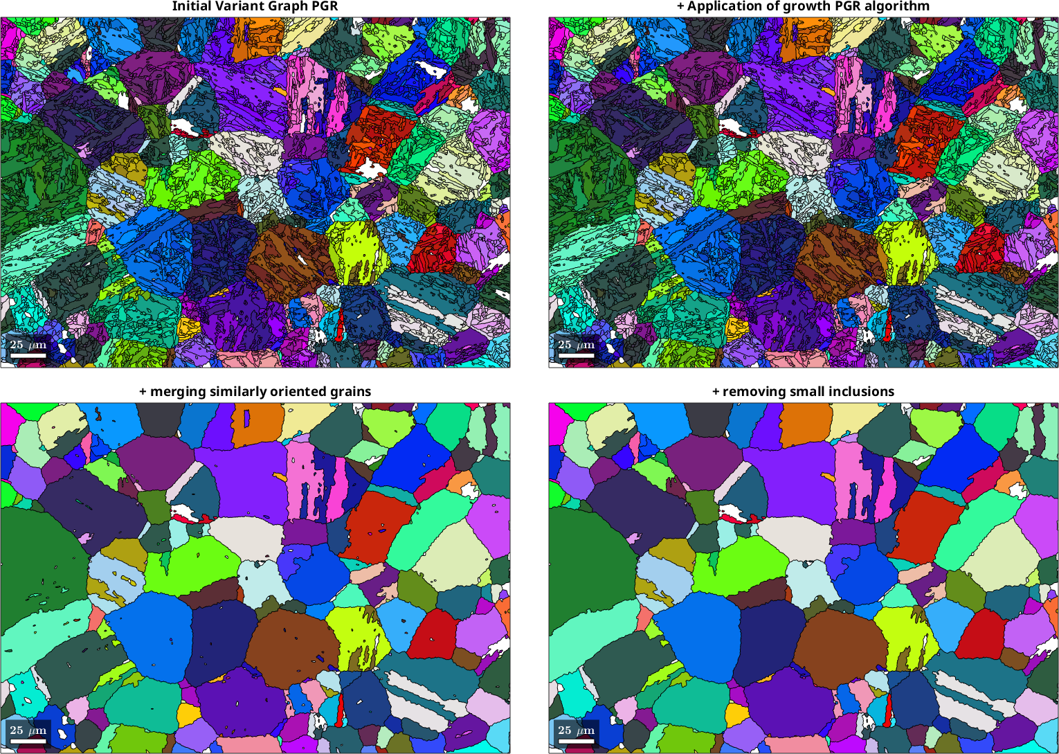
It may not be entirely possible to judge the quality of the PGR with having access to a validation dataset (i.e. without knowing the actual parent microstructure), nevertheless some observations can be made: An inflation power of 1.2 seems to be too high, leading to large patches of material that have not been reconstructed. A good indicator for the present microstructure is to check in how far likely annealing twins have been resolved with a realistic morphology and how very small parent grains may become present that are unlikely to be associated with real parent grains. Based on this the choice of an inflation power of 1.05 and numIter of 10 seems to be a good choice, although it is hard to make an objective assessment. Note that an inflation power of 1 means that no clustering is enforced - with this setting the algorithm simply explores the local neighborhood up to the degree of neighbor defined by numIter and bases the most likely parent orientation on the overall probabilities within this region.
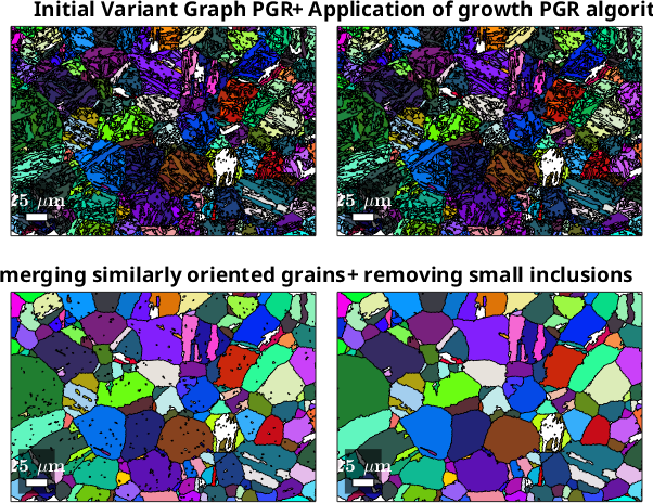
Final reconstruction
We can now do the final reconstruction using the optimized parameters and subsequently apply a growth-based PGR algorithm to reconstruct the remaining grains, as well as some post-processing steps to clean up the microstructure. You may also want to play with the parameter minProb of the calcParentFromVote method, which defines the minimum probability for a specific parent orientation required to conduct the PGR of a specific child grain. Lowering this parameter will lead to a more complete, but less confident PGR.
% *** PGR using the Variant Graph Approach
% setup the variant graph
job.calcVariantGraph('threshold',2.5*degree,'tolerance',2.5*degree)
% Cluster the variant graph with different parameters
job.clusterVariantGraph('inflationPower',1.05,'numIter',10);
% Calculate the parent grain orientations
job.calcParentFromVote('minProb',0.5);
% Plot the PGR result (before any cleaning is applied)
figure;
f(8) = newMtexFigure('layout',[2,2],'Name','Final PGR with cleaning procedure');
plot(job.parentGrains,job.parentGrains.meanOrientation);
title("Initial Variant Graph PGR")
nextAxis;
% *** Growth algorithm to fill non-reconstructed regions based on
% previously reconstructed neighboring austenite orientations
% Calculate new Votes for all parent-child grain combinations. Iterate a
% few times
for ii = 1:5
job.calcGBVotes('p2c','reconsiderAll');
job.calcParentFromVote('minProb',0.5);
end
% Plot the PGR result (before any cleaning is applied)
plot(job.parentGrains,job.parentGrains.meanOrientation);
title("+ Application of growth PGR algorithm")
nextAxis;
% *** Merge neighboring grains with low parent grain misorientation
% Merge neighboring parent grains that have <= 7.5°
% misorientation angle to each other
job.mergeSimilar('threshold',7.5*degree);
% Plot the PGR result after merging similarly oriented grains
plot(job.parentGrains,job.parentGrains.meanOrientation);
title("+ merging similarly oriented grains")
nextAxis;
% *** Remove small inclusion grains
% Merge inclusion grains with a size <= 100 into the host grains
job.mergeInclusions('maxSize',100);
% Plot the PGR result after merging inclusions
plot(job.parentGrains,job.parentGrains.meanOrientation);
title("+ removing small inclusions")ans = parentGrainReconstructor
phase mineral symmetry grains area reconstructed
parent Iron fcc 432 0 0% 0%
child Iron bcc (old) 432 9338 100%
OR: (347.2°,9°,56.8°)
c2c fit: 1.2°, 1.6°, 2°, 2.7° (quintiles)
closest ideal OR: (111) || (011) [1-10] || [100] fit: 2.4°
variant graph: 438720 entries
Warning: grains.grainSize is depreciated. Please use
grains.numPixel instead
Warning: grains.grainSize is depreciated. Please use
grains.numPixel instead
Warning: grains.grainSize is depreciated. Please use
grains.numPixel instead
Warning: grains.grainSize is depreciated. Please use
grains.numPixel instead
Warning: grains.grainSize is depreciated. Please use
grains.numPixel instead
Warning: grains.grainSize is depreciated. Please use
grains.numPixel instead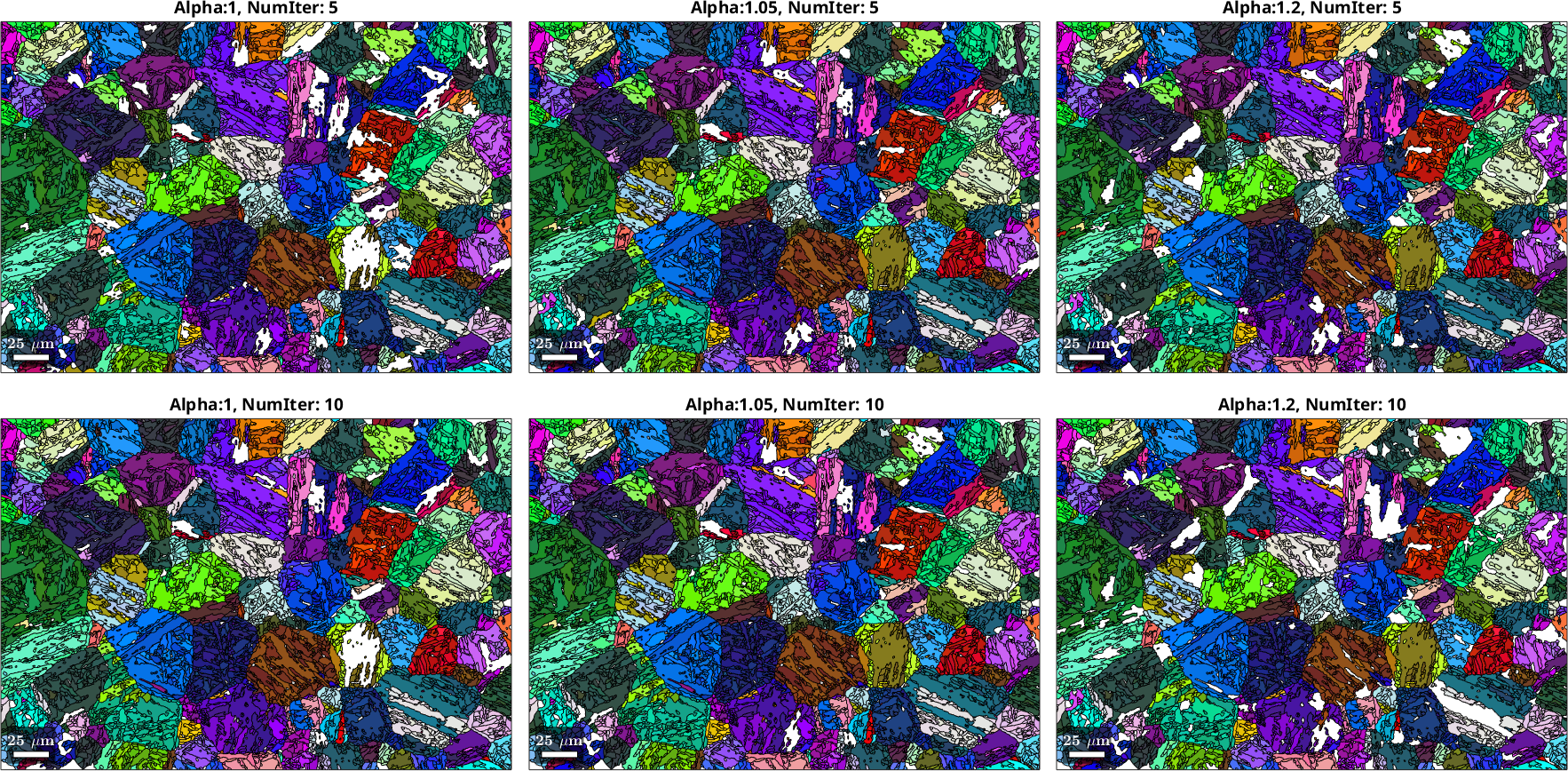
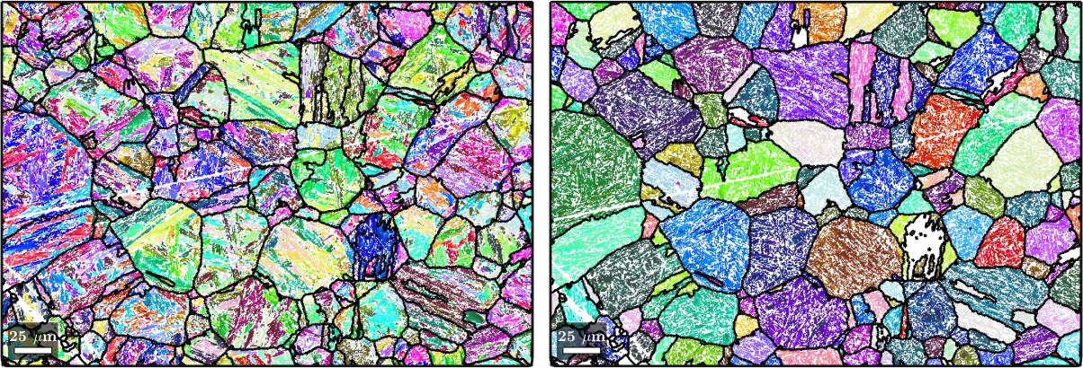
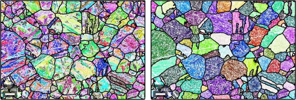
We are now finished with the PGR and can, as a last step, plot the child and reconstructed parent EBSD data overlayed with the outlines of the parent grains.
% Prepare plotting
figure;
f(8) = newMtexFigure('layout',[1,2]);

% Plot the initial orientation data with the prior parent grain outlines
plot(job.ebsdPrior,job.ebsdPrior.orientations);
hold on
plot(job.grains.boundary,'lineWidth',2)
hold off

% Plot the reconstructed orientation data with the prior parent grain outlines
nextAxis;
parentEBSD = job.calcParentEBSD;
plot(parentEBSD(job.csParent),parentEBSD(job.csParent).orientations);
hold on
plot(job.grains.boundary,'lineWidth',2)
hold off