Seismic velocities and anisotropy - single crystal plots edit page

Plot 2D velocity surfaces - phase, slowness and wavefront - for a given plane normal direction, for example xvector, yvector or zvector. The material is stishovite (SiO2) at high pressure.

David Mainprice 1/05/2018

The Elastic Stiffness Tensor of Stishovite

Reference: Elastic constants Stishovite, Weidner et al 1982 JGR
Reference: Crystal Structure Sinclair and Ringwood 78 Nature P422
d=4.2901

% Define density (g/cm3)
 rho= 4.2901;

% elastic Cij stiffness tensor (GPa) as matrix M
 M = ...
 [[  453.00  211.00  203.00    0.00    0.00    0.00];...
 [   211.00  453.00  203.00    0.00    0.00    0.00];...
 [   203.00  203.00  776.00    0.00    0.00    0.00];...
 [     0.00    0.00    0.00  252.00    0.00    0.00];...
 [     0.00    0.00    0.00    0.00  252.00    0.00];...
 [     0.00    0.00    0.00    0.00    0.00  302.00]];

% define cartesian tensor crystal crystalSymmetry & frame
cs_Tensor = crystalSymmetry('4/mmm',[  4.9133  4.9133  5.4048],...
 [  90.0000  90.0000  90.0000]*degree,'x||a','z||c',...
 'mineral','Stishovite 1982');
%
% define elastic stiffness tensor Cijkl
C = stiffnessTensor(M,cs_Tensor,'density',rho);

compute wave velocities and polarization directions

% the propagation direction is just the vector normal to the sphere
prop = S2AxisFieldHarmonic.normal;

% the wave velocities and polarization directions as directional dependend
% functions
[vp,vs1,vs2,pp,ps1,ps2] = velocity(C);

Plotting settings

% plane normal direction for 2d sections
planeNormal = vector3d.Z;

% plotting convention - plot X-axis to east
plotx2east;

% close all open graphics
close all

% some global options for the titles
%titleOpt = {'FontSize',getMTEXpref('FontSize'),'visible','on','color','k'};
titleOpt = {'FontSize',25};
% option for legend
legendOpt = {'location','best'};
% option for mtexColorbar
ColorbarOpt = {'location','southoutside'};
% options for sections
optSec = {'color','interp','linewidth',5,'doNotDraw'};
% options for quiver
optQuiver = {'linewidth',5,'autoScaleFactor',0.25,'doNotDraw'};
% options for prop
optQuiverProp = {'color','k','linewidth',2,'autoScaleFactor',0.15,'doNotDraw'};

1: Phase velocity surface (km/s)

figure(1)

% phase velocities
plotSection(vp,planeNormal,optSec{:})
hold on
plotSection(vs1,planeNormal,optSec{:})
plotSection(vs2,planeNormal,optSec{:})

% polarization directions
quiverSection(vp,pp,planeNormal,'color','c',optQuiver{:})
quiverSection(vs1,ps1,planeNormal,'color','g',optQuiver{:})
quiverSection(vs2,ps2,planeNormal,'color','m',optQuiver{:})

% plot propagation directions as reference
quiverSection(vp,prop,planeNormal,optQuiverProp{:})
quiverSection(vs1,prop,planeNormal,optQuiverProp{:})
quiverSection(vs2,prop,planeNormal,optQuiverProp{:})

axis off tight
legend('Vp','Vs1','Vs2','pp','ps1','ps2','X',legendOpt{:})
mtexTitle('Phase velocity surfaces (km/s)',titleOpt{:})

% seismic velocity slow = red 2 blue =fast
mtexColorMap red2blue
mtexColorbar('Title','(km/s)',ColorbarOpt{:})

% Az El for planeNormal = Z
%view(0,85)
hold off
drawNow(gcm,'figSize','large')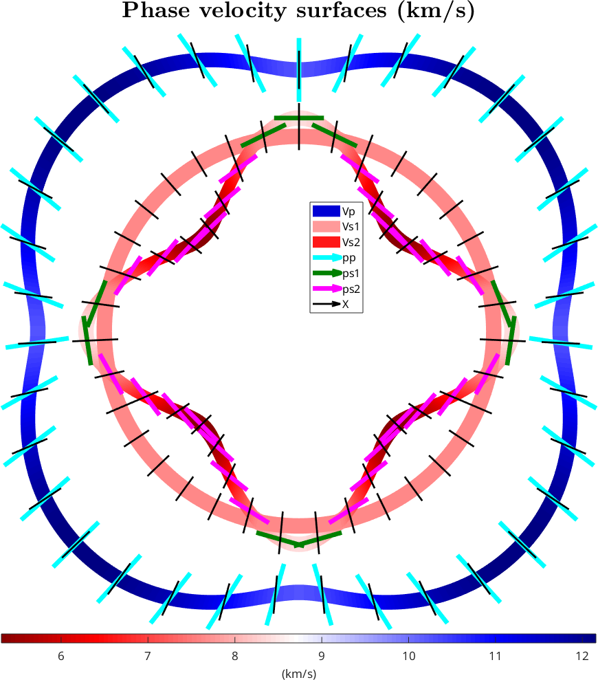

2: Slowness surface (s/km)

figure(2)

% slowness
plotSection(1./vp,planeNormal,optSec{:})
hold on
plotSection(1./vs1,planeNormal,optSec{:})
plotSection(1./vs2,planeNormal,optSec{:})

% polarization directions
quiverSection(1./vp,pp,planeNormal,'color','c',optQuiver{:})
quiverSection(1./vs1,ps1,planeNormal,'color','g',optQuiver{:})
quiverSection(1./vs2,ps2,planeNormal,'color','m',optQuiver{:})

% plot propagation directions as reference
quiverSection(1./vp,prop,planeNormal,optQuiverProp{:})
quiverSection(1./vs1,prop,planeNormal,optQuiverProp{:})
quiverSection(1./vs2,prop,planeNormal,optQuiverProp{:})

axis off tight
legend('Vp','Vs1','Vs2','pp','ps1','ps2','X',legendOpt{:})
mtexTitle('Slowness surfaces (s/km)',titleOpt{:})

% seismic slowness slow = blue 2 red =fast
mtexColorMap blue2red
mtexColorbar('Title','(s/km)',ColorbarOpt{:})

% Az El for planeNormal = Z
%view(0,85)
hold off
drawNow(gcm,'figSize','large')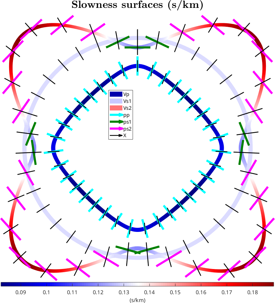

Select the two S-waves (Vs1 and Vs2 where Vs1>Vs2 in velocity)

by the orientation of the polarization vectors ps1 and ps2 with respect to the specimen Z direction, so that sv (v=vertical) is the S-wave with polarization closest to Z, while sh (h=horizontal) has the polarization closest to the plane normal to Z. Both pairs of polarizations, (sv,sh) and (ps1,ps2), are orthogonal.

which values to switch this defines a function which is either one or zero

id = angle(ps1,vector3d.Z) <= 89.9*degree;
vsv = id .* vs1 + (1-id) .* vs2;
vsh = id .* vs2 + (1-id) .* vs1;
psv = id .* ps1 + (1-id) .* ps2;
psh = id .* ps2 + (1-id) .* ps1;

3: Phase velocity surface (km/s) with vs1 & vs2

figure(1)
% phase velocities
plotSection(vp,planeNormal,optSec{:})
hold on
plotSection(vs1,planeNormal,optSec{:})
plotSection(vs2,planeNormal,optSec{:})

% polarization directions
quiverSection(vp,pp,planeNormal,'color','c',optQuiver{:})
quiverSection(vs1,ps1,planeNormal,'color','g',optQuiver{:})
quiverSection(vs2,ps2,planeNormal,'color','m',optQuiver{:})

% plot propagation directions as reference
quiverSection(vp,prop,planeNormal,optQuiverProp{:})
quiverSection(vs1,prop,planeNormal,optQuiverProp{:})
quiverSection(vs2,prop,planeNormal,optQuiverProp{:})

axis off tight
legend('Vp','Vs1','Vs2','pp','ps1','ps2','X',legendOpt{:})
mtexTitle('Phase velocity surfaces (km/s)',titleOpt{:})

mtexColorMap blue2red
mtexColorbar('Title','(km/s)',ColorbarOpt{:})

% Az El for planeNormal = Z
%view(0,85)
hold off
drawNow(gcm,'figSize','large')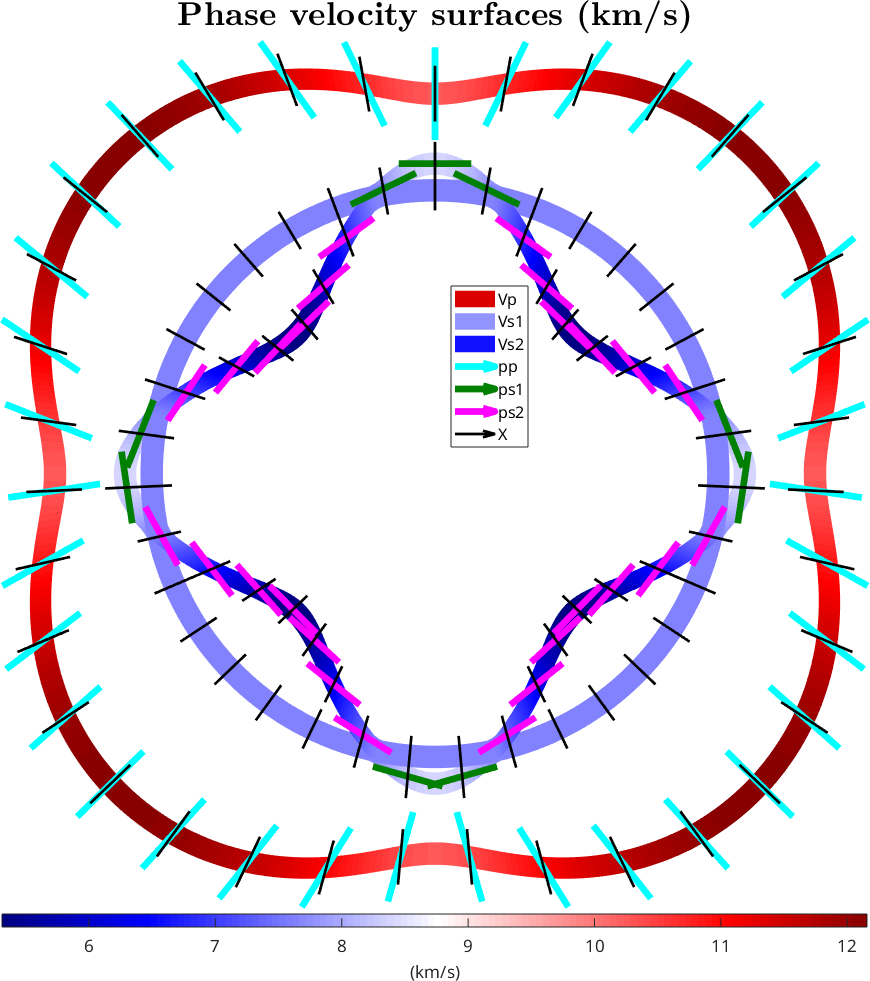

4: Phase velocity surface (km/s) with vsv & vsh

figure(2)
% phase velocities
plotSection(vp,planeNormal,optSec{:})
hold on
plotSection(vsv,planeNormal,optSec{:})
plotSection(vsh,planeNormal,optSec{:})

% polarization directions
quiverSection(vp,pp,planeNormal,'color','c',optQuiver{:})
quiverSection(vsv,ps1,planeNormal,'color','g',optQuiver{:})
quiverSection(vsh,ps2,planeNormal,'color','m',optQuiver{:})

% plot propagation directions as reference
quiverSection(vp,prop,planeNormal,optQuiverProp{:})
quiverSection(vsv,prop,planeNormal,optQuiverProp{:})
quiverSection(vsh,prop,planeNormal,optQuiverProp{:})

axis off tight
legend('Vp','Vsv','Vsh','pp','ps1','ps2','X',legendOpt{:})
mtexTitle('Phase velocity surfaces (km/s)',titleOpt{:})

mtexColorMap blue2red
mtexColorbar('Title','(km/s)',ColorbarOpt{:})

% Az El for planeNormal = Z
%view(0,85)
hold off
drawNow(gcm,'figSize','large')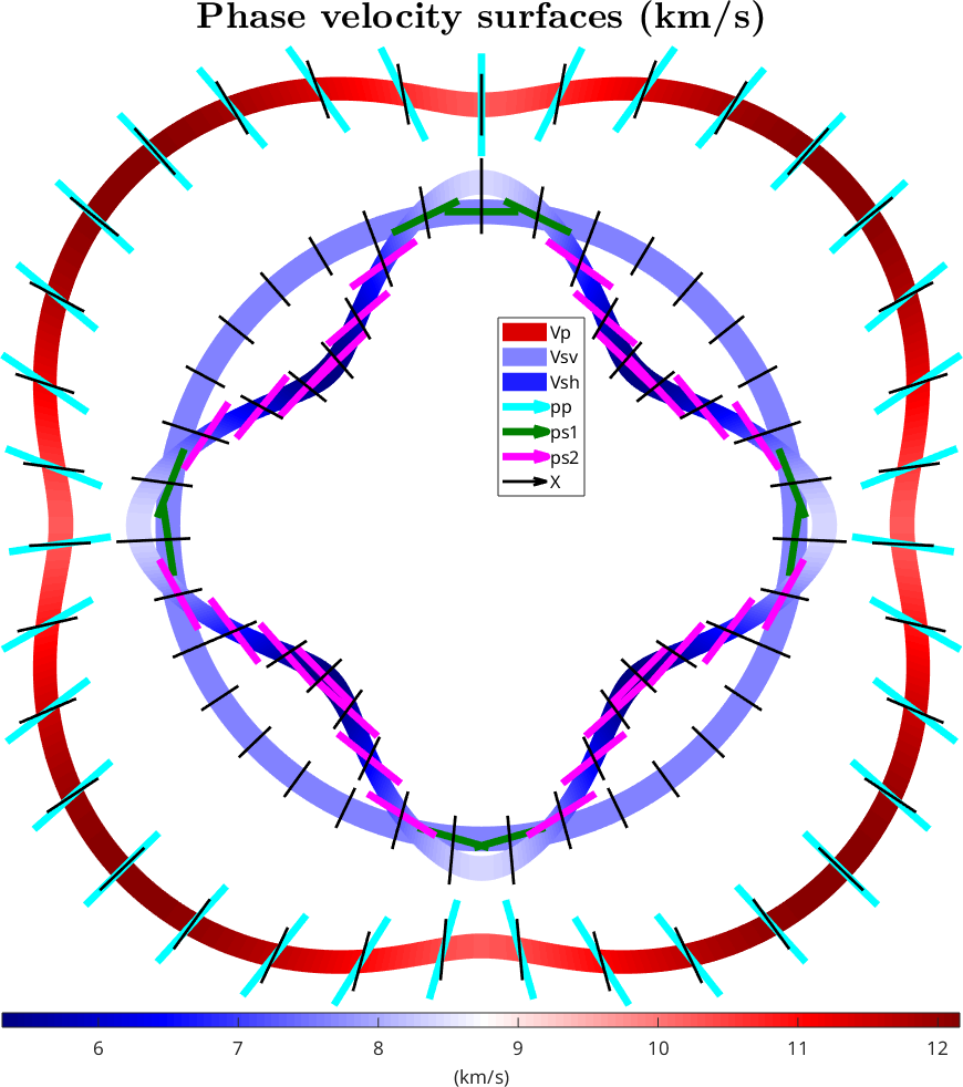

5: plot slowness in plane normal Z

figure(3)
plotSection(1./vp,planeNormal,optSec{:})
hold on
plotSection(1./vs1,planeNormal,optSec{:})
plotSection(1./vs2,planeNormal,optSec{:})

% polarization vectors pp,ps1,ps2
quiverSection(1./vp,pp,planeNormal,'color','c',optQuiver{:})
quiverSection(1./vs1,ps1,planeNormal,'color','g',optQuiver{:})
quiverSection(1./vs2,ps2,planeNormal,'color','m',optQuiver{:})

% propagation vectors (prop)
quiverSection(1./vp,prop,planeNormal,optQuiverProp{:})
quiverSection(1./vs1,prop,planeNormal,optQuiverProp{:})
quiverSection(1./vs2,prop,planeNormal,optQuiverProp{:})

axis off tight
legend('Sp','Ss1','Ss2','pp','ps1','ps2','X',legendOpt{:})
mtexTitle('Stishovite : Slowness surfaces (s/km)',titleOpt{:})
% seismic slowness slow = blue 2 red =fast
mtexColorMap red2blue
mtexColorbar('Title','(s/km)',ColorbarOpt{:})

hold off
drawNow(gcm,'figSize','large')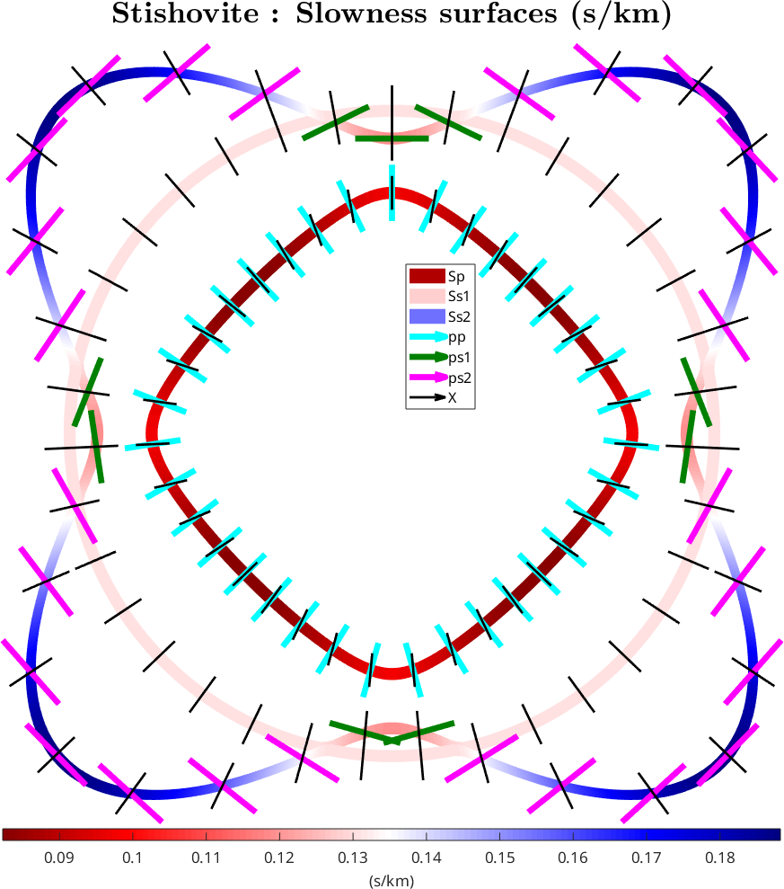

Compute WaveFront as spherical functions: EnergyVectors Evp, Evs1 & Evs2

Evp = energyVector(C,[],vp,pp);
Evs1 = energyVector(C,[],vs1,ps1);
Evs2 = energyVector(C,[],vs2,ps2);

plot wavefront in plane normal Z

close all

% Vp,Vs1,Vs2 wavefronts with motif
%optSec = {'linewidth',5,'doNotDraw'};
optSec = {'color','interp','linewidth',2,'doNotDraw'};
plotSection(Evp,planeNormal,optSec{:})
hold on
plotSection(Evs1,planeNormal,optSec{:})
plotSection(Evs2,planeNormal,optSec{:})
%
% polarization vectors pp,ps1,ps2
quiverSection(Evp,Evp,planeNormal,'color','c',optQuiver{:})
quiverSection(Evs1,Evs1,planeNormal,'color','g',optQuiver{:})
quiverSection(Evs2,Evs2,planeNormal,'color','m',optQuiver{:})

% propagation vectors (prop)
quiverSection(Evp,prop,planeNormal,optQuiverProp{:})
quiverSection(Evs1,prop,planeNormal,optQuiverProp{:})
quiverSection(Evs2,prop,planeNormal,optQuiverProp{:})

axis off tight
legend('Evp','Evs1','Evs2','pp','ps1','ps2','X',legendOpt{:})
mtexTitle('Stishovite : Wavefront surfaces (km/s)',titleOpt{:})

mtexColorbar('Title','(km/s)',ColorbarOpt{:})

hold off
drawNow(gcm,'figSize','large')

% End of demo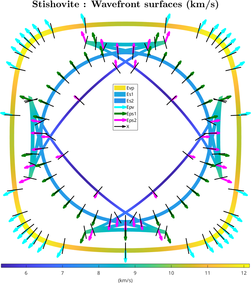

Citing this page. This page is part of the documentation of MTEX, a free and open source MATLAB toolbox for analyzing and modeling crystallographic textures. It was written by The MTEX Developers and is published at https://mtex-toolbox.github.io/ExSeismicVelocitySingleCrystalDemo2d.html. If you use MTEX, or reuse text or figures from this page, in your research, please cite

F. Bachmann, R. Hielscher, H. Schaeben: Texture Analysis with MTEX - Free and Open Source Software Toolbox, Solid State Phenomena 160 (2010), 63-68. 10.4028/www.scientific.net/SSP.160.63

BibTeX

@article{bachmann2010mtex,
  author  = {F. Bachmann and R. Hielscher and H. Schaeben},
  title   = {Texture Analysis with MTEX - Free and Open Source Software Toolbox},
  journal = {Solid State Phenomena},
  volume  = {160},
  pages   = {63-68},
  year    = {2010},
  doi     = {10.4028/www.scientific.net/SSP.160.63},
  url     = {https://doi.org/10.4028/www.scientific.net/SSP.160.63}
}

Other papers describing specific MTEX methods are listed under Publications — please cite the one that best fits your application. The MTEX source code is licensed under the GNU General Public License v2.0; the text and figures of this documentation are licensed under CC BY 4.0, which permits reuse — including by automated systems — provided The MTEX Developers and this page are credited.