ODF Reconstruction from X-Ray Diffraction Data of an Al Alloy Rolled Sheet

ODF Reconstruction from X-Ray Diffraction Data of an Al Alloy Rolled Sheet edit page author:

Import the Data

The following pole figure intensities have been measured by a Philips X'Pert diffractometer using Cu-Kalpha radiation. The sample comes from a commercial aluminum alloy (AA6061-T4) sheet of 0.9 mm thickness. Scans were done over the RD-TD plane of the sheet (RD//X; TD//Y; ND//Z). The tree main FCC poles for XRD were scanned, i.e., {1 1 1}, {2 0 0}, {2 2 0}.

% Lets import the raw data

% crystal symmetry
CS = crystalSymmetry('m-3m', [1 1 1],'mineral','Al');

% create a Pole Figure variable containing the data
fname = fullfile(mtexExamplePath,'ExODFReconstruction','data','alt4_*.rw1');
pf = PoleFigure.load(fname,CS,'interface','rw1');

plot(pf, 'colorrange', 'tight', 'minmax')
mtexColorMap WhiteJet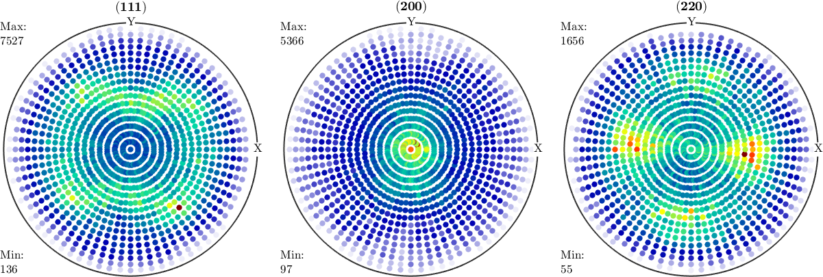

Background and Defocusing Correction

When working with X-ray diffraction the intensities are usually corrupted by background radiation as well as a decay of the intensities towards the equator. This effect can somehow be estimated by measuring an untextured powder sample. In the present case the following powder intensities were determined.

% the powder intensities for {1 1 1}, {2 0 0}, {2 2 0}
h = Miller({1 1 1}, {2 0 0}, {2 2 0},CS);
y = {...
  [684,697,656,647,684,641,637,694,623,664,679,632,595,515,560,416,421,343]
  [684,697,656,647,684,641,637,694,623,664,679,632,595,515,560,416,421,343];
  [460,422,411,472,403,421,465,447,511,427,497,457,409,407,341,309,234,160]
  };

% the measurement grid
S2G = regularS2Grid('points', [1,18], 'antipodal');

Lets store these intensities in variables of type PoleFigure.

mtt = 2;    % time per measurement point of each PF scan
mtb = 30;   % time for the full circle (azimutal angle) of defocusing scan

% create background and defocusing pole figures
pf_bg = PoleFigure(h, S2G, y, CS);
pf_def = pf_bg ./ max(pf_bg);
pf_bg = pf_bg * mtt / mtb;

plot(pf_def)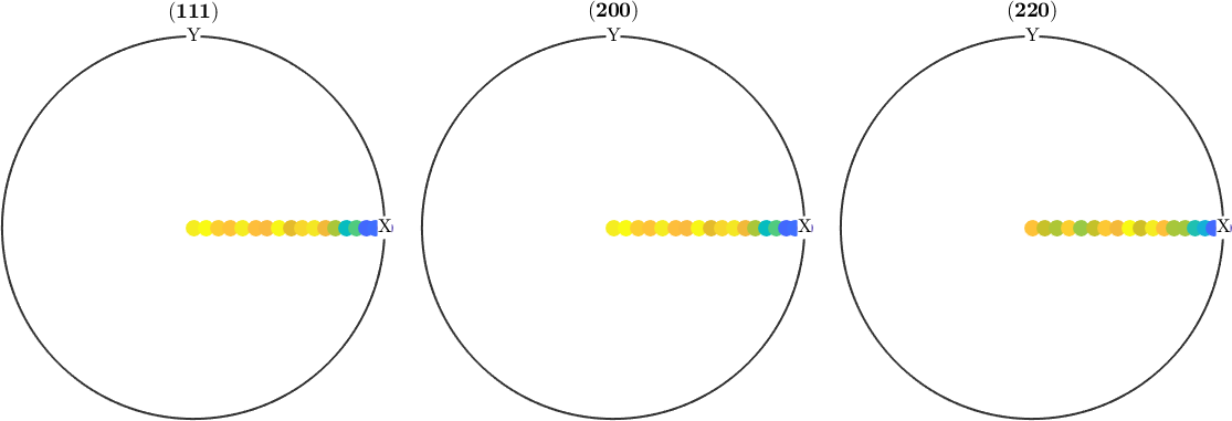

For background and defocusing correction we subtract the background and divide by the defocusing factor.

% perform background and defocusing correction
pf = (pf - pf_bg) ./ pf_def;

Despite the defocusing correction the intensities at larger polar angles are very off, lets simply remove them.

pf(pf.r.theta >= 70*degree) = [];

plot(pf, 'minmax')
mtexColorMap WhiteJet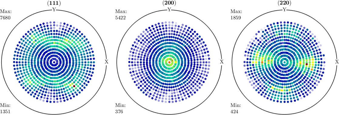

ODF computation

Using the corrected XRD data we may now compute an ODF using the command calcODF.

solver = MLSSolver(pf,'halfwidth',5*degree,'resolution',2.5*degree,...
  'intensityWeights');

odf = solver.calcODF;

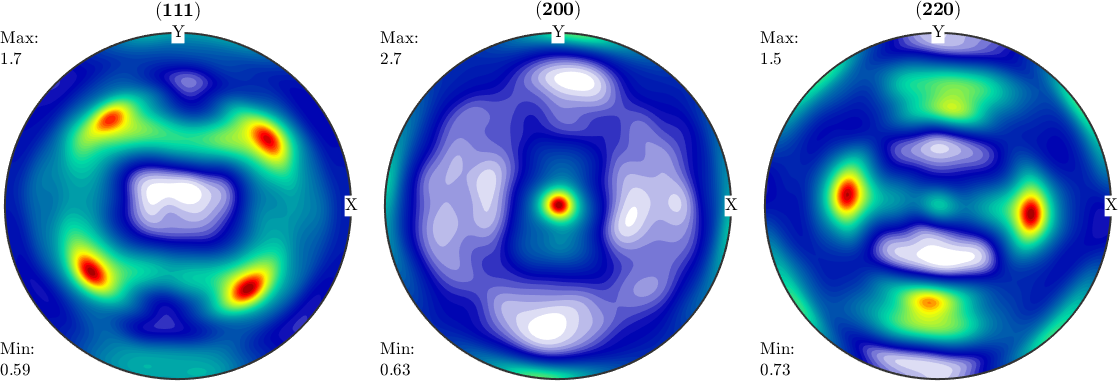
plotPDF(odf, h, 'minmax')

% This texture shows the typically dominant 'cube' orientation due to
% recrystallization after rolling of Al alloy plates and sheets.
% There's a slight misalignment of the sample's orthotropy axes wrt the
% X-Y directions. This is due to a small deviation of the sample when
% positioned on the goniometer of the X-ray diffractometer.