
This example demonstrates how to convert SKAT time of flight neutron intensities into pole figure intensities.
In a time of flight experiment every detector records a full diffraction spectrum at once, with each Bragg reflection appearing as a peak at its own flight time. A pole figure is obtained by integrating one peak over all specimen directions, so the work is: read the spectra, subtract the background, integrate each peak, and hand the resulting intensities to PoleFigure together with the specimen directions they were measured in.
Step 1: Import and Analyze the Spectra
The SKAT goniometer carries 19 detectors spread over polar angles from 0 to 90 degrees, and turns the specimen into 72 azimuthal positions, giving 19 x 72 spectra per measurement cycle. loadallspectra reads all of them from one directory, and calc_background estimates the background that sits underneath the peaks.
% import all spectra
spec = loadallspectra(fullfile(mtexExamplePath,'ExODFReconstruction','Knie_10','Knie_10'));

% compute background
bg = calc_background(spec);

% plot the first spectrum together with its background. Drop the
% |noInteraction| flag to browse through all detectors and phi positions
% with the arrow keys - that waits for key presses, so it cannot be used
% while publishing this page.
plot_spectra(spec,bg,'noInteraction')
load detector: a, b, c, d, e, f, g, h, i, j, k, l, m, n, o, p, q, r, s, .
calculate background: .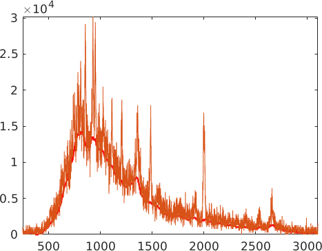
Step 2: Peak Detection and Integration
Each peak that is to become a pole figure needs an integration window, given below as a pair of time of flight channels. There are nine of them here, so nine pole figures come out at the end.
Which reflection sits in which window is read from quartz.txt, a table of Miller indices and structure factors shipped with MTEX in tools/dubna_tools. sfpos maps rows of that table onto the nine windows. Several rows for one window mean several reflections overlap there and cannot be separated - the resulting pole figure is then a superposition, and the structure factors collected in c are the weights with which the individual reflections contribute to it.
% Range fits measure period in '2005'. One row per peak, giving the
% integration window in time of flight channels.
peakrange = [2509 2550;...
  1981 2009;...
  1470 1500;...
  1366 1390;...
  1344 1366;...
  1280 1295;...
  1196 1211;...
  1103 1117;...
  1015 1030];

% specify crystal and specimen symmetry
CS = crystalSymmetry('-3m',[4.9,4.9,5.4]);

% file with structure factors for quartz
sf = txt2mat('quartz.txt');

% which rows of the structure factor file belong to which peak - a cell
% entry with several rows is a superposed reflection
sfpos  = {1,[2 3],4,[5 6],7,8,[9,10],11,[13,14]};

for k = 1:length(sfpos)
  i = sfpos{k};
  h{k} = Miller(sf(i,2),sf(i,3),sf(i,4),sf(i,5),CS);
  c{k} = sf(i,end).';
end


% extract peaks and calculate spectra sums
[sumdetectr,sumphi,sumspectr,peaks,peaksbg] = proceed_spectra(spec,bg,300:1200,peakrange);
************
* quartz.txt
* read mode: auto
* 83 data lines analysed
* 0 header line(s)
* 12 data column(s)
* 0 string replacement(s)
************Step 3: Set up the Pole Figures
All nine pole figures were measured in the same specimen directions - the 19 detector rings times 72 rotations of the goniometer - so one grid is built once and shared by all of them. Then one PoleFigure per peak is assembled from that grid and the integrated intensities, and pf.c attaches the superposition weights collected above.
r = DubnaGrid(19);

pf = PoleFigure(h{1},r,fliplr(squeeze(peaks(1,:,:))),CS);

for k = 2:length(h)

  pf({k}) = PoleFigure(h{k}.',r,fliplr(squeeze(peaks(k,:,:))),CS);

end

pf.c = c;

%plot(rotate(pf,rotation.byAxisAngle(xvector,90*degree)))
plot(pf)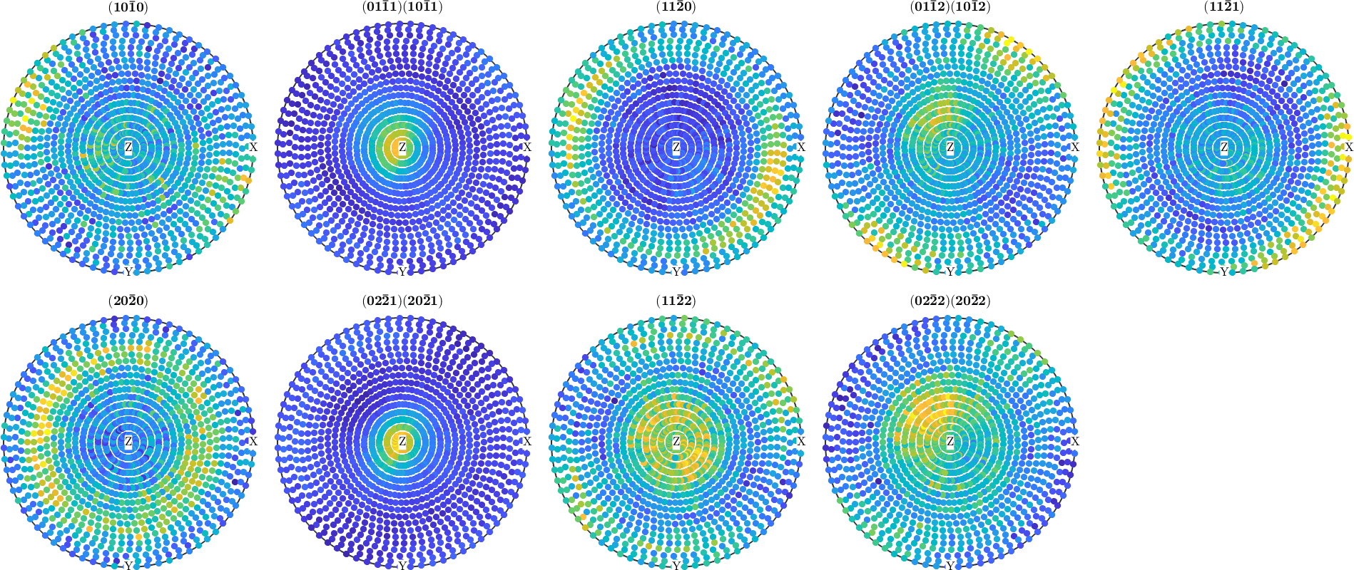
Citing this page.
This page is part of the documentation of
MTEX, a free and open
source MATLAB toolbox for analyzing and modeling crystallographic textures.
It was written by The MTEX Developers and is published at
https://mtex-toolbox.github.io/TOF2PoleFigure.html.
If you use MTEX, or reuse text or figures from this page, in your research,
please cite
F. Bachmann, R. Hielscher, H. Schaeben: Texture Analysis with MTEX - Free and Open Source Software Toolbox, Solid State Phenomena 160 (2010), 63-68. 10.4028/www.scientific.net/SSP.160.63
BibTeX
@article{bachmann2010mtex,
  author  = {F. Bachmann and R. Hielscher and H. Schaeben},
  title   = {Texture Analysis with MTEX - Free and Open Source Software Toolbox},
  journal = {Solid State Phenomena},
  volume  = {160},
  pages   = {63-68},
  year    = {2010},
  doi     = {10.4028/www.scientific.net/SSP.160.63},
  url     = {https://doi.org/10.4028/www.scientific.net/SSP.160.63}
}
Other papers describing specific MTEX methods are listed under Publications — please cite the one that best fits your application. The MTEX source code is licensed under the GNU General Public License v2.0; the text and figures of this documentation are licensed under CC BY 4.0, which permits reuse — including by automated systems — provided The MTEX Developers and this page are credited.