Slip System Analysis in \(\alpha\)-Alumina edit page author: Ruben Wagner, Robert Lehnert, TU Bergakademie Freiberg, Institute of Materials Engineering, Germany

Data Import

The following EBSD map has been measured by Ruben Wagner TUBAF, Institute of Materials Engineering, 2022 within the project SFB 920. It shows an alumina inclusion in 42CrMo4 steel after nanoindentation.

% set crystal symmetry
cs = crystalSymmetry.load('Al2O3-Corundum.cif');

% set plotting convention
setMTEXpref('xAxisDirection','east');
setMTEXpref('zAxisDirection','intoPlane');

% import data
path = [mtexExamplePath filesep 'ExPlasticity' filesep ];
ebsd = EBSD.load([path 'K1_C_16_EBSD_original_bc.txt'],...
  'CS',{'notIndexed',cs,'notIndexed'},'radiant');

% rotate the data in the right reference frame
rot = rotation.byEuler(90*degree,180*degree,0*degree);
ebsd = rotate(ebsd('indexed'),rot,'keepXY');

Initial grain reconstruction and visualization

% reconstruct grain structure
[grains,ebsd.grainId] = calcGrains(ebsd,'angle',1*degree);

cKey = ipfColorKey(cs);
cKey.inversePoleFigureDirection = vector3d(1,0,0);

figure(2)
plot(ebsd,cKey.orientation2color(ebsd.orientations))
hold on
plot(grains.boundary,grains.boundary.misrotation.angle./degree,'linewidth',3)
hold off
mtexColorbar

Warning: The syntax

  [grains,ebsd.grainId] = calcGrains(ebsd)

has been replaced by

  [grains,ebsd] = calcGrains(ebsd)

It still works, but is deprecated. Switch this warning off by

  warning('off','MTEX:calcGrains:oldSyntax')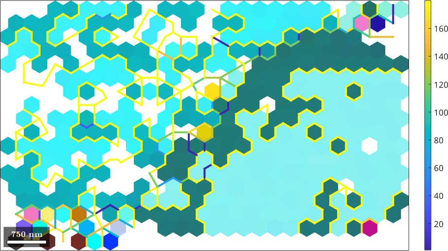

Correct for misindexing due to pseudosymmetry

Looking at the raw data we observe several neighbouring measurements that are exactly 180 degree rotated with respect to each other. This is indicated by color coded grain boundaries. It is suspected that this misorientation occurs as the EBSD system has a hard time to distinguish the Kikuchi pattern of two orientations that differ by a rotation about the c-axis by 180 degree.

In order to correct for this misindexing we proceed as follows

# Identify grain boundaries due to pseudo symmetry
# Merge grains with common pseudo symmetry grain boundaries and
compute the dominant orientation of the merged grains
# Correct the EBSD data according to the pseudo symmetry

1. Identify boundaries between pseudosymmetric grains

% all Corundum Corundum boundaries
gB = grains.boundary('indexed');

% define the pseudo symmetry
pseudoSym = orientation.byAxisAngle(cs.cAxis,180*degree);

% allow for a 3 degree threshold
ispseudoBnd = angle(gB.misorientation,pseudoSym)<3*degree;

2. Merge grains with common pseudo symmetry grain boundaries This results in two big grains as visualised below

[grains, parentId] = grains.merge(gB(ispseudoBnd),'calcMeanOrientation',...
  @(g) updateOri(g,pseudoSym));

plot(grains,cKey.orientation2color(grains.meanOrientation))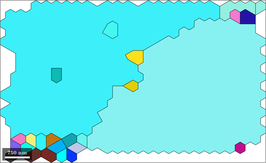

3. Correct the EBSD data according to the pseudo symmetry

% find all EBSD data which differ by the computed grain orientation by
% about 180 degree
flipPseudo = ~(angle(ebsd.orientations,grains(parentId(ebsd.grainId)).meanOrientation)> 10*degree);

ebsd(flipPseudo).orientations = ebsd(flipPseudo).orientations * pseudoSym;

cKey.inversePoleFigureDirection = zvector;
plot(ebsd,cKey.orientation2color(ebsd.orientations))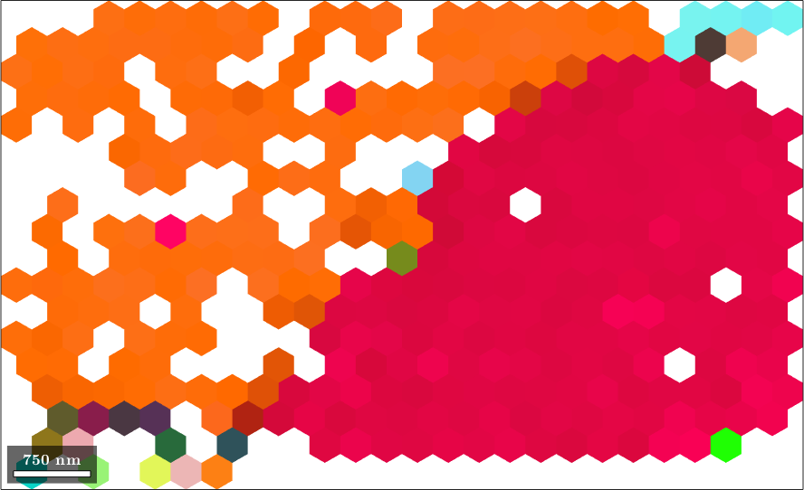

Data cleaning

We perform some more data cleaning steps including

removing too small grains
filling of the not indexed pixels

% redo grain reconstruction
[grains,ebsd.grainId] = calcGrains(ebsd,'angle',1*degree);

% and remove little grains
ebsd(grains(grains.numPixel<4)) = [];
[grains,ebsd.grainId] = calcGrains(ebsd,'angle',1*degree);

% filling EBSD holes
F = halfQuadraticFilter;
F.alpha=0.3;
ebsdS = smooth(ebsd,F,'fill',grains);

% visualize the result
cKey.inversePoleFigureDirection = zvector;
plot(ebsdS,cKey.orientation2color(ebsdS.orientations))

hold on
plot(ebsd, ebsd.bc,'FaceAlpha',0.3)
colormap gray % make the image grayscale
mtexColorbar
hold off

Warning: The syntax

  [grains,ebsd.grainId] = calcGrains(ebsd)

has been replaced by

  [grains,ebsd] = calcGrains(ebsd)

It still works, but is deprecated. Switch this warning off by

  warning('off','MTEX:calcGrains:oldSyntax')
 
Warning: The syntax

  [grains,ebsd.grainId] = calcGrains(ebsd)

has been replaced by

  [grains,ebsd] = calcGrains(ebsd)

It still works, but is deprecated. Switch this warning off by

  warning('off','MTEX:calcGrains:oldSyntax')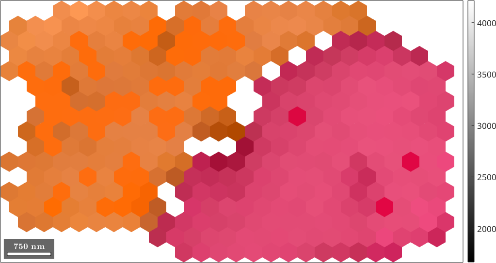

Schmid Factor Analysis

Next we compute the active slip system during pressure in z-direction. The possible dominant slip systems in alumina are described in Mao2011 and 2012 as

n = Miller(1,0,-1,1,cs,'HKIL');
b = Miller(-1,2,-1,0,cs,'UVTW');
sS = slipSystem(b,n)

sS = slipSystem (Corundum)
 
   U    V    T    W  | H    K    I    L CRSS
  -1    2   -1    0    1    0   -1    1    1

Next we determine the Schmid factor for all symmetrically equivalent slip systems.

% rotate symmetrically equivalent slip systems into specimen coordinates of
% each grain
sSLocal = grains.meanOrientation * sS.symmetrise('antipodal');

% compute Schmid factor according Z axis
sigma = stressTensor.uniaxial(vector3d.Z);
SF = abs(sSLocal.SchmidFactor(sigma));

% sort the slips system according to their Schmid factor from largest to
% smallest
[SF, reorder] = sort(SF,2,"descend");
reorder = sub2ind(size(reorder),repmat((1:size(reorder,1))',1,size(reorder,2)),reorder);
sSLocal = sSLocal(reorder);

Finally, we plot the trace of the slip planes together with the slip direction in the EBSD map.

figure(2)
cKey.inversePoleFigureDirection = zvector;
plot(ebsdS,cKey.orientation2color(ebsdS.orientations))

hold on
plot(ebsd, ebsd.bc,'FaceAlpha',0.3)
colormap gray % make the image grayscale
hold off

order = 1;

hold on
% visualize the trace of the slip plane
quiver(grains,sSLocal(:,order).trace,'color','blue','linewidth',5)

% and the slip direction
quiver(grains,sSLocal(:,order).b,'color','gray','linewidth',5)

hold off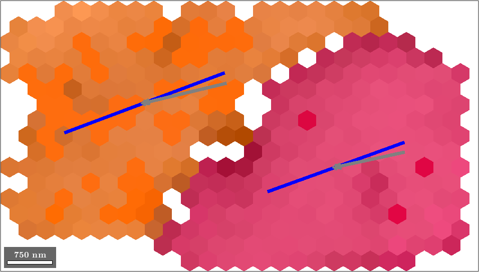

function ori = updateOri(grains,pseudoSym)

ori = grains.meanOrientation;

cId = 1+calcCluster(ori,'weights',grains.numPixel);

% variant 1
[~,isTrue] = max(accumarray(cId(:),grains.numPixel));

% variant 2
%[~,isTrue] = max(accumarray(cId(:),grains.numNeighbors));

ori(cId ~= isTrue) = ori(cId ~= isTrue) * pseudoSym;

ori = mean(ori,'weights',grains.numPixel,'robust');

end

References

Ruben Wagner, Robert Lehnert, Enrico Storti, Lisa Ditscherlein, Christina Schröder, Steffen Dudczig, Urs A. Peuker, Olena Volkova, Christos G. Aneziris, Horst Biermann, Anja Weidner, Nanoindentation of alumina and multiphase inclusions in 42CrMo4 steel, 2022.

Citing this page. This page is part of the documentation of MTEX, a free and open source MATLAB toolbox for analyzing and modeling crystallographic textures. It was written by The MTEX Developers and is published at https://mtex-toolbox.github.io/ExSlipSystemAlumina.html. If you use MTEX, or reuse text or figures from this page, in your research, please cite

F. Bachmann, R. Hielscher, H. Schaeben: Texture Analysis with MTEX - Free and Open Source Software Toolbox, Solid State Phenomena 160 (2010), 63-68. 10.4028/www.scientific.net/SSP.160.63

BibTeX

@article{bachmann2010mtex,
  author  = {F. Bachmann and R. Hielscher and H. Schaeben},
  title   = {Texture Analysis with MTEX - Free and Open Source Software Toolbox},
  journal = {Solid State Phenomena},
  volume  = {160},
  pages   = {63-68},
  year    = {2010},
  doi     = {10.4028/www.scientific.net/SSP.160.63},
  url     = {https://doi.org/10.4028/www.scientific.net/SSP.160.63}
}

Other papers describing specific MTEX methods are listed under Publications — please cite the one that best fits your application. The MTEX source code is licensed under the GNU General Public License v2.0; the text and figures of this documentation are licensed under CC BY 4.0, which permits reuse — including by automated systems — provided The MTEX Developers and this page are credited.