
Calculating and plotting elastic velocities from elastic stiffness tensor \(C_{ijkl}\) and density (by David Mainprice).
Crystal Symmetry and definition of the elastic stiffness tensor
crystal symmetry - Orthorhombic mmm Olivine structure (4.7646 10.2296 5.9942 90.00 90.00 90.00)
cs_tensor = crystalSymmetry('mmm',[4.7646,10.2296,5.9942],...
  'x||a','z||c','mineral','Olivine');
Import 4th rank tensor as 6 by 6 matrix
Olivine elastic stiffness (Cij) tensor in GPa Abramson E.H., Brown J.M., Slutsky L.J., and Zaug J.(1997) The elastic constants of San Carlos olivine to 17 GPa. Journal of Geophysical Research 102: 12253-12263.
Enter tensor as 6 by 6 matrix M, line by line.
M = [[320.5  68.15  71.6     0     0     0];...
    [ 68.15  196.5  76.8     0     0     0];...
    [  71.6   76.8 233.5     0     0     0];...
    [   0      0      0     64     0     0];...
    [   0      0      0      0    77     0];...
    [   0      0      0      0     0  78.7]];

% Define density (g/cm3)
rho=3.355;

% Define tensor object in MTEX
% Cij -> Cijkl - elastic stiffness tensor
C = stiffnessTensor(M,cs_tensor,'density',rho)
C = stiffnessTensor (Olivine)
density: 3.355
unit : GPa
rank : 4 (3 × 3 × 3 × 3)
tensor in Voigt matrix representation:
320.5 68.2 71.6 0 0 0
68.2 196.5 76.8 0 0 0
71.6 76.8 233.5 0 0 0
0 0 0 64 0 0
0 0 0 0 77 0
0 0 0 0 0 78.7Compute seismic velocities as functions on the sphere
[vp,vs1,vs2,pp,ps1,ps2] = C.velocity('harmonic');Plotting section
Here we set preference for a nice plot.
% set color map to seismic color map: blue2redColorMap
setMTEXpref('defaultColorMap',blue2redColorMap)

% some options
blackMarker = {'Marker','s','MarkerSize',10,'antipodal',...
  'MarkerEdgeColor','white','MarkerFaceColor','black','doNotDraw'};
whiteMarker = {'Marker','o','MarkerSize',10,'antipodal',...
  'MarkerEdgeColor','black','MarkerFaceColor','white','doNotDraw'};

% some global options for the titles
%titleOpt = {'FontSize',getMTEXpref('FontSize'),'visible','on'}; %{'FontSize',15};
titleOpt = {'visible','on','color','k'};

% Setup multiplot
% define plot size [origin X,Y,Width,Height]
mtexFigure('position',[0 0 1000 1000]);

% set up spacing between subplots default is 10 pixel
%mtexFig.innerPlotSpacing = 20;

% Standard Seismic plot with 8 subplots in 3 by 3 matrix
%
% Plot matrix layout
%        1 Vp        2 AVs      3 S1 polarization
%        4 Vs1       5 Vs2      6 dVs
%        7 Vp/Vs1    8 Vp/Vs2
%
Vp : Plot P-wave velocity (km/s)
% Plot P-wave velocity (km/s)
plot(vp,'contourf','complete','upper','noLabel')
mtexTitle('Vp (km/s)',titleOpt{:})

% extrema
[maxVp, maxVpPos] = max(vp);
[minVp, minVpPos] = min(vp);

% percentage anisotropy
AVp = 200*(maxVp-minVp) / (maxVp+minVp);

% mark maximum with black square and minimum with white circle
hold on
plot(maxVpPos.symmetrise,blackMarker{:})
plot(minVpPos.symmetrise,whiteMarker{:})
hold off

% subTitle
xlabel(['Vp Anisotropy = ',num2str(AVp,'%6.1f')],titleOpt{:})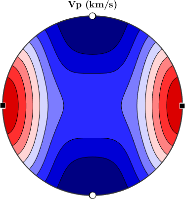
AVs : Plot S-wave anisotropy percentage for each propagation direction
defined as AVs = 200*(Vs1-Vs2)/(Vs1+Vs2)
% create a new axis
nextAxis

% Plot S-wave anisotropy (percent)
AVs = 200*(vs1-vs2)./(vs1+vs2);
plot(AVs,'contourf','complete','upper');
mtexTitle('S-wave anisotropy (%)',titleOpt{:})

% Max percentage anisotropy
[maxAVs,maxAVsPos] = max(AVs);
[minAVs,minAVsPos] = min(AVs);

xlabel(['Max Vs Anisotropy = ',num2str(maxAVs,'%6.1f')],titleOpt{:})

% mark maximum with black square and minimum with white circle
hold on
plot(maxAVsPos.symmetrise,blackMarker{:})
plot(minAVsPos.symmetrise,whiteMarker{:})
hold off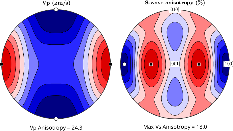
S1 Polarization: Plot fastest S-wave (Vs1) polarization directions
% create a new axis
nextAxis

plot(AVs,'contourf','complete','upper','noLabel');
mtexTitle('Vs1 polarization',titleOpt{:})

hold on
plot(ps1,'linewidth',2,'color','black','doNotDraw')
hold off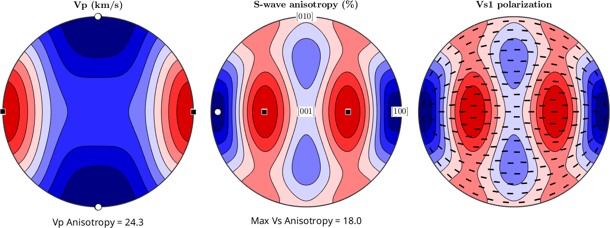
Vs1 : Plot Vs1 velocities (km/s)
% create a new axis
nextAxis

plot(vs1,'contourf','doNotDraw','complete','upper','noLabel');
mtexTitle('Vs1 (km/s)',titleOpt{:})

% Percentage anisotropy
[maxS1,maxS1pos] = max(vs1);
[minS1,minS1pos] = min(vs1);
AVs1=200*(maxS1-minS1)./(maxS1+minS1);

xlabel(['Vs1 Anisotropy = ',num2str(AVs1,'%6.1f')],titleOpt{:})

hold on
plot(ps1,'linewidth',2,'color','black')

% mark maximum with black square and minimum with white circle
plot(maxS1pos.symmetrise,blackMarker{:})
plot(minS1pos.symmetrise,whiteMarker{:})
hold off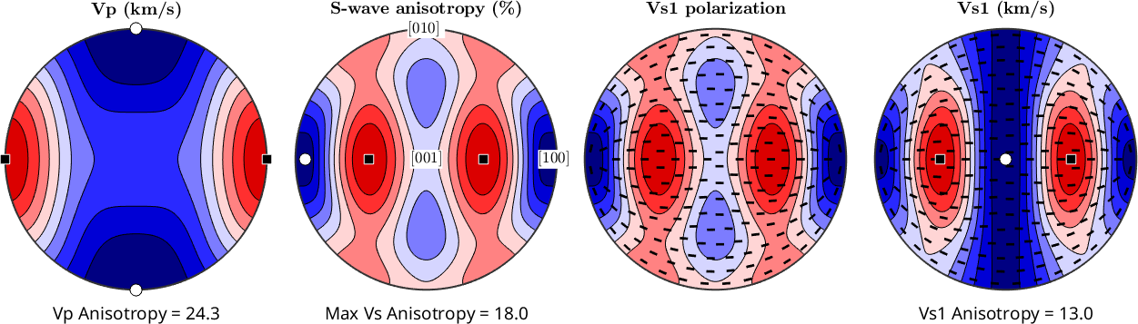
Vs2 : Plot Vs2 velocities (km/s)
% create a new axis
nextAxis

plot(vs2,'contourf','doNotDraw','complete','upper','noLabel');
mtexTitle('Vs2 (km/s)',titleOpt{:})

% Percentage anisotropy
[maxS2,maxS2pos] = max(vs2);
[minS2,minS2pos] = min(vs2);
AVs2=200*(maxS2-minS2)./(maxS2+minS2);
xlabel(['Vs2 Anisotropy = ',num2str(AVs2,'%6.1f')],titleOpt{:})

hold on
plot(ps2,'linewidth',2,'color','black')

% mark maximum with black square and minimum with white circle
plot(maxS2pos.symmetrise,blackMarker{:})
plot(minS2pos.symmetrise,whiteMarker{:})
hold off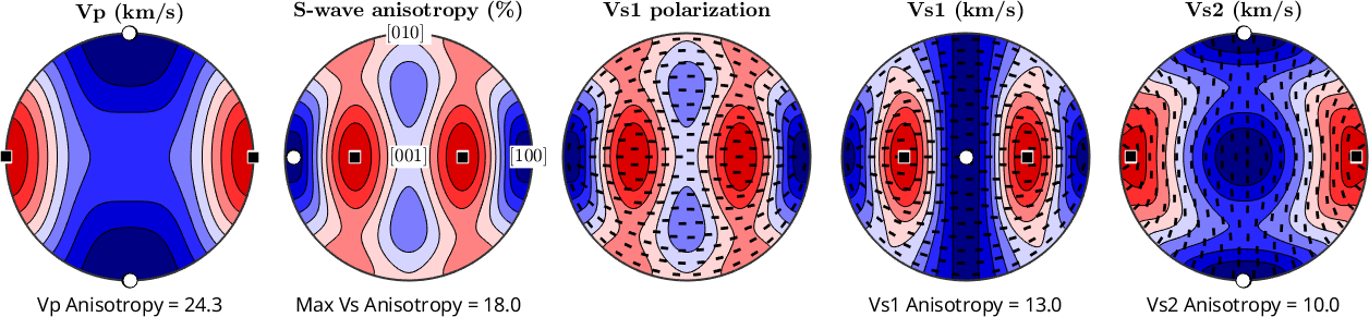
dVs : Plot Velocity difference Vs1-Vs2 (km/s) plus Vs1 polarization
% create a new axis
nextAxis

dVs = vs1-vs2;
plot(dVs,'contourf','complete','upper','noLabel');
mtexTitle('dVs=Vs1-Vs2 (km/s)',titleOpt{:})

% Max percentage anisotropy
[maxdVs,maxdVsPos] = max(dVs);
[mindVs,mindVsPos] = min(dVs);

xlabel(['Max dVs (km/s) = ',num2str(maxdVs,'%6.2f')],titleOpt{:})

% mark maximum with black square and minimum with white circle
hold on
plot(maxdVsPos.symmetrise,blackMarker{:})
plot(mindVsPos.symmetrise,whiteMarker{:})
hold off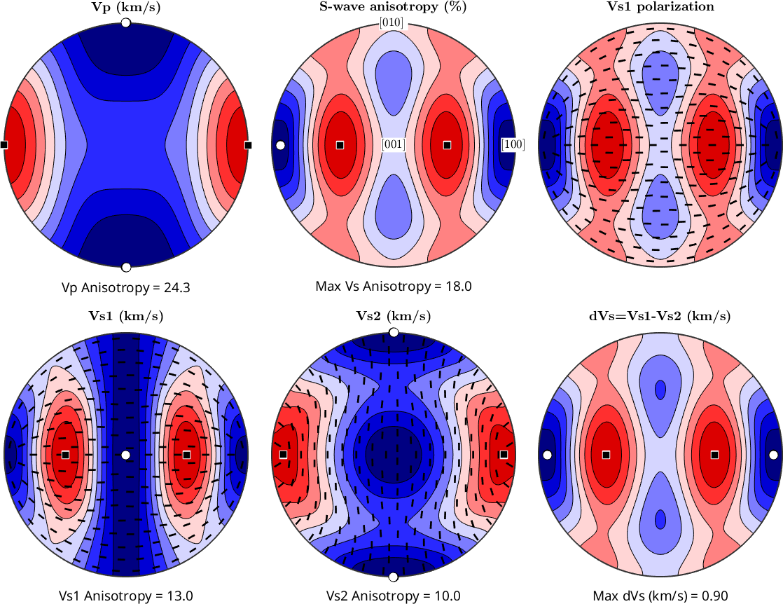
Vp/Vs1 : Plot Vp/Vs1 ratio (no units)
% create a new axis
nextAxis

vpvs1 = vp./vs1;
plot(vpvs1,'contourf','complete','upper','noLabel');
mtexTitle('Vp/Vs1',titleOpt{:})

% Percentage anisotropy
[maxVpVs1,maxVpVs1Pos] = max(vpvs1);
[minVpVs1,minVpVs1Pos] = min(vpvs1);
AVpVs1=200*(maxVpVs1-minVpVs1)/(maxVpVs1+minVpVs1);

xlabel(['Vp/Vs1 Anisotropy = ',num2str(AVpVs1,'%6.1f')],titleOpt{:})

% mark maximum with black square and minimum with white circle
hold on
plot(maxVpVs1Pos.symmetrise,blackMarker{:})
plot(minVpVs1Pos.symmetrise,whiteMarker{:})
hold off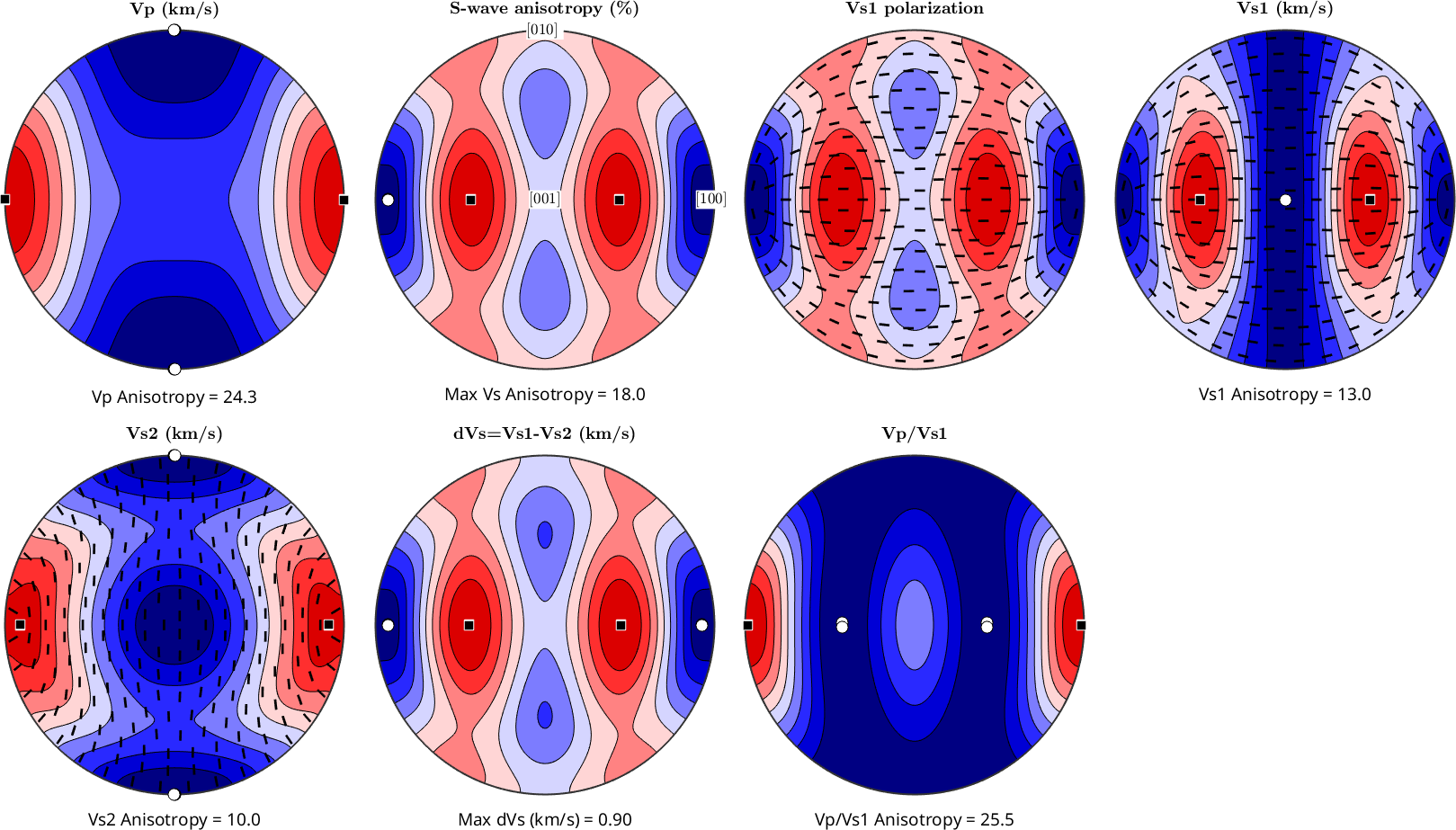
Vp/Vs2 : Plot Vp/Vs2 ratio (no units)
% create a new axis
nextAxis

vpvs2 = vp./vs2;
plot(vpvs2,'contourf','complete','upper','noLabel');
mtexTitle('Vp/Vs2',titleOpt{:})

% Percentage anisotropy
[maxVpVs2,maxVpVs2Pos] = max(vpvs2);
[minVpVs2,minVpVs2Pos] = min(vpvs2);
AVpVs2=200*(maxVpVs2-minVpVs2)/(maxVpVs2+minVpVs2);

xlabel(['Vp/Vs2 Anisotropy = ',num2str(AVpVs2,'%6.1f')],titleOpt{:})

% mark maximum with black square and minimum with white circle
hold on
plot(maxVpVs2Pos.symmetrise,blackMarker{:})
plot(minVpVs2Pos.symmetrise,whiteMarker{:})
hold off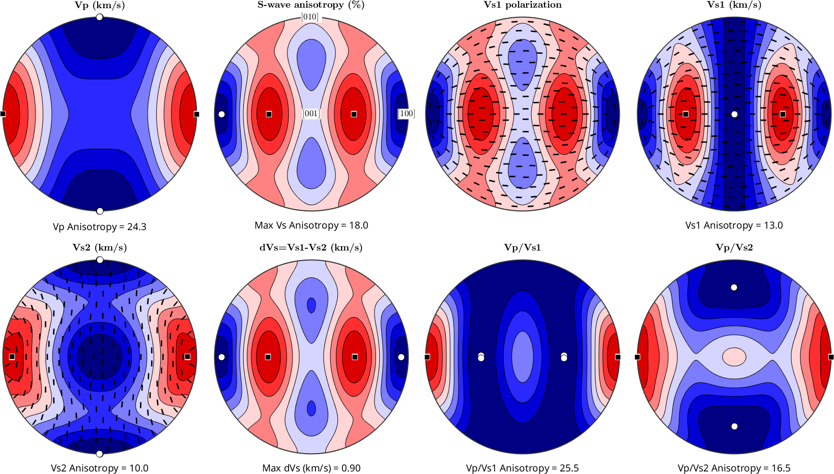
% add colorbars to all plots
mtexColorbar
drawNow(gcm,'figSize','large')

% reset old colormap
setMTEXpref('defaultColorMap',WhiteJetColorMap)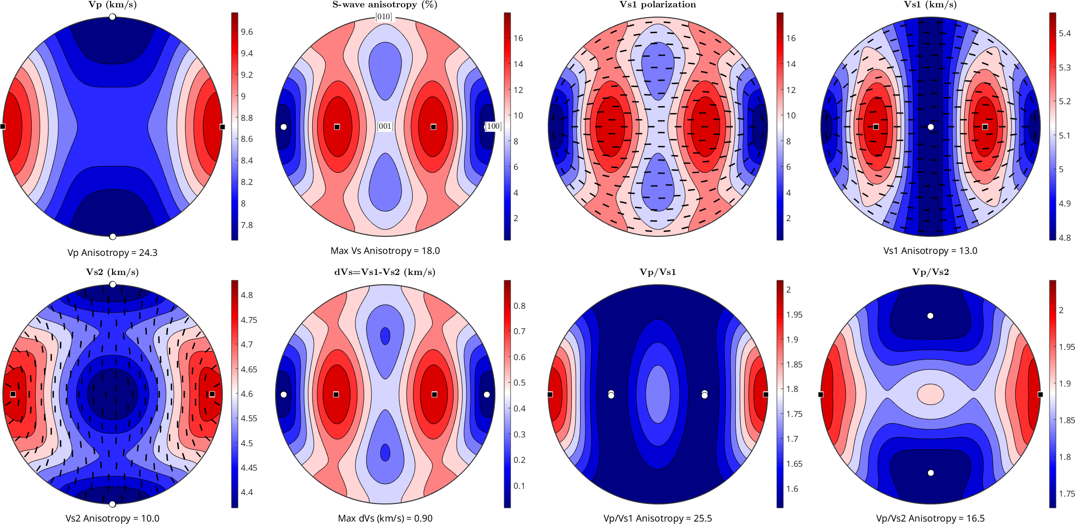
Citing this page.
This page is part of the documentation of
MTEX, a free and open
source MATLAB toolbox for analyzing and modeling crystallographic textures.
It was written by The MTEX Developers and is published at
https://mtex-toolbox.github.io/ExSeismicPlots.html.
If you use MTEX, or reuse text or figures from this page, in your research,
please cite
F. Bachmann, R. Hielscher, H. Schaeben: Texture Analysis with MTEX - Free and Open Source Software Toolbox, Solid State Phenomena 160 (2010), 63-68. 10.4028/www.scientific.net/SSP.160.63
BibTeX
@article{bachmann2010mtex,
  author  = {F. Bachmann and R. Hielscher and H. Schaeben},
  title   = {Texture Analysis with MTEX - Free and Open Source Software Toolbox},
  journal = {Solid State Phenomena},
  volume  = {160},
  pages   = {63-68},
  year    = {2010},
  doi     = {10.4028/www.scientific.net/SSP.160.63},
  url     = {https://doi.org/10.4028/www.scientific.net/SSP.160.63}
}
Other papers describing specific MTEX methods are listed under Publications — please cite the one that best fits your application. The MTEX source code is licensed under the GNU General Public License v2.0; the text and figures of this documentation are licensed under CC BY 4.0, which permits reuse — including by automated systems — provided The MTEX Developers and this page are credited.