
the elastic stiffness C, sigma = C : eps; a 6 x 6 Voigt matrix in GPa or the full array
Input
M |
6-by-6 Voigt matrix, full (…, 3, 3, 3, 3) coefficients, or another tensor |
args |
optional reference frame |
kwargs |
tensor constructor options, including density, frame, unit and Kelvin; unit defaults to ‘GPa’ |
Example
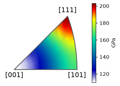
Construct an illustrative cubic stiffness tensor in GPa, rotate it into specimen coordinates, and compare Young’s modulus along the same physical direction before and after rotation.
import numpy as np
import matplotlib.pyplot as plt
from mtex import (crystalFrame, stiffnessTensor, orientation, Miller, degree,
                  plot, mtexColorbar)

cs = crystalFrame('m-3m')
C = stiffnessTensor([[200, 120, 120, 0, 0, 0],
                     [120, 200, 120, 0, 0, 0],
                     [120, 120, 200, 0, 0, 0],
                     [0, 0, 0, 80, 0, 0],
                     [0, 0, 0, 0, 80, 0],
                     [0, 0, 0, 0, 0, 80]], cs, unit='GPa')
direction = Miller(1, 0, 0, cs, 'uvw')
ori = orientation.byEuler(30*degree, 40*degree, 20*degree, cs)
rotated = ori * C
print('Crystal direction modulus (GPa):', round(float(C.YoungsModulus(direction)), 3))
print('Rotated direction modulus (GPa):', round(float(rotated.YoungsModulus(ori*direction)), 3))
plot(C.YoungsModulus(), resolution=5*degree)
mtexColorbar(title='GPa')
plt.show()
The two numerical values agree because tensor and direction were rotated together. The plot shows the directional variation for these model coefficients, not measured material data.
Crystal direction modulus (GPa): 110.0
Rotated direction modulus (GPa): 110.0
Members
| bulkModulus | the bulk modulus of an isotropic polycrystal, the Voigt and Reuss bounds |
| ChristoffelTensor | the elastic Christoffel tensor for a wave propagation direction |
| colon | the double contraction A : B, the last two indices of A against the first two of B, MATLAB’s A:B |
| energyVector | the energy velocity of a lossless elastic plane wave, the vector C_ijkl p_j n_k p_l / (rho v) |
| hashinShtrikmanBounds | the Hashin-Shtrikman bounds of the isotropic moduli, the tightest pair for a quasihomogeneous polycrystal: (lower=(K, G), upper=(K, G)), each the extreme estimate over the references whose residual is semidefinite, found on the boundary of that convex set by a golden section over the shear and a bisection over the bulk modulus |
| HashinShtrikmanModulus | the Hashin-Shtrikman estimate of the isotropic moduli of a polycrystal from a reference medium K0, G0, over arrays of references: the bulk and shear moduli, and the definiteness of C - C0 (1 where the estimate is a lower bound, -1 an upper one, 0 where it is neither and the moduli are NaN) |
| inv | the inverse: rank two by the matrix, rank four through the Voigt matrix, which swaps the convention and with it the class, a stiffness inverting to a compliance |
| linearCompressibility | the linear compressibility, the length change per pressure in the direction v, S_ijkk v_i v_j |
| mtimes | scale a tensor, multiply rank-two tensors, or contract an elastic tensor with a strain |
| plotSeismicVelocities | the overview of the seismic wave velocities of a stiffness tensor, six pole figures |
| PoissonRatio | the Poisson ratio of the tension direction x and the transverse direction y, minus the transverse over the longitudinal strain, -S_ijkl x_i x_j y_k y_l / S_mnop x_m x_n x_o x_p |
| rand | a random tensor with the symmetries its class and frame ask for |
| shearModulus | the shear modulus of the plane h and the shear direction u, 1 / (4 S_ijkl h_i u_j h_k u_l) |
| stiffnessTensor | the elastic stiffness C, sigma = C : eps |
| velocity | the speeds of the three elastic plane waves in a direction and their polarisations, the eigenvalues and eigenvectors of the Christoffel tensor |
| volumeCompressibility | the volume change per pressure, S_iikk |
| YoungsModulus | Young’s modulus in the direction v, the reciprocal of S_ijkl v_i v_j v_k v_l |
Used on
DefinitionAsCoordinateTransform, CPOSeismicProperties, IsotropicTheory, TensorAverage, TensorDefinition
MATLAB’s stiffnessTensor_index
source
Citing this page.
This page is part of the documentation of
MTEX, a free and open
source MATLAB toolbox for analyzing and modeling crystallographic textures.
It was written by The MTEX Developers and is published at
https://mtex-toolbox.github.io/stiffnessTensor_index_py.html.
If you use MTEX, or reuse text or figures from this page, in your research,
please cite
F. Bachmann, R. Hielscher, H. Schaeben: Texture Analysis with MTEX - Free and Open Source Software Toolbox, Solid State Phenomena 160 (2010), 63-68. 10.4028/www.scientific.net/SSP.160.63
BibTeX
@article{bachmann2010mtex,
  author  = {F. Bachmann and R. Hielscher and H. Schaeben},
  title   = {Texture Analysis with MTEX - Free and Open Source Software Toolbox},
  journal = {Solid State Phenomena},
  volume  = {160},
  pages   = {63-68},
  year    = {2010},
  doi     = {10.4028/www.scientific.net/SSP.160.63},
  url     = {https://doi.org/10.4028/www.scientific.net/SSP.160.63}
}
Other papers describing specific MTEX methods are listed under Publications — please cite the one that best fits your application. The MTEX source code is licensed under the GNU General Public License v2.0; the text and figures of this documentation are licensed under CC BY 4.0, which permits reuse — including by automated systems — provided The MTEX Developers and this page are credited.