Isotropic Theory

An isotropic material has the same elastic response in every direction. Its stiffness therefore needs only two independent numbers. A general anisotropic stiffness tensor needs as many as 21.

The engineering moduli are different ways to choose those two numbers. They include the shear and bulk moduli, Young’s modulus, Poisson’s ratio, and the Lame constants.

This page starts from one anisotropic crystal and makes an isotropic aggregate from randomly oriented copies. It then shows how to read, compare, and convert the resulting moduli.

import matplotlib.pyplot as plt
import numpy as np

from mtex import *

Start with an anisotropic crystal

Albite is triclinic and is about as anisotropic as a common mineral gets. Its density is in g/cm3, and its stiffness entries are in GPa.

rho = 2.6230

# crystal symmetry and crystal frame
cs = crystalFrame('-1', [8.290, 12.966, 7.151], np.array([91.18, 116.31, 90.14]) * degree, 'x||a*', 'y||b',
                  mineral='An0 Albite 2016')

# stiffness tensor
C = stiffnessTensor(
  [[68.30, 32.20, 30.40, 4.90, -2.30, -0.90],
   [32.20, 184.30, 5.00, -4.40, -7.70, -6.40],
   [30.40, 5.00, 180.00, -9.20, 7.50, -9.40],
   [4.90, -4.40, -9.20, 25.00, -2.40, -7.20],
   [-2.30, -7.70, 7.50, -2.40, 26.90, 0.60],
   [-0.90, -6.40, -9.40, -7.20, 0.60, 33.60]],
  cs, density=rho)

Average a random aggregate

A material made of these crystals in random orientations is isotropic. The orientation distribution function (ODF) records the volume fraction at each orientation. A uniform ODF represents the random orientation distribution used here.

Random orientations do not determine one exact aggregate stiffness. The result also depends on how the grains are arranged. The Voigt model assumes uniform strain and gives an upper bound. The Reuss model assumes uniform stress and gives a lower bound. The Hill estimate is the arithmetic mean of those two tensors.

C_iso_Voigt, C_iso_Reuss, C_iso_Hill = mean(C, uniformODF(C.CS), 'all')
C_iso_Voigt

stiffnessTensor (y↓→x)
  density: 2.623
  unit   : GPa
  rank   : 4 (3 × 3 × 3 × 3)
  tensor in Voigt matrix representation
  118.3333   35.4667   35.4667        0        0        0
   35.4667  118.3333   35.4667        0        0        0
   35.4667   35.4667  118.3333        0        0        0
         0         0         0  41.4333        0        0
         0         0         0        0  41.4333        0
         0         0         0        0        0  41.4333

C_iso_Reuss

stiffnessTensor (y↓→x)
  density: 2.623
  unit   : GPa
  rank   : 4 (3 × 3 × 3 × 3)
  tensor in Voigt matrix representation
  93.8309  34.1599  34.1599        0        0        0
  34.1599  93.8309  34.1599        0        0        0
  34.1599  34.1599  93.8309        0        0        0
        0        0        0  29.8355        0        0
        0        0        0        0  29.8355        0
        0        0        0        0        0  29.8355

C_iso_Hill

stiffnessTensor (y↓→x)
  density: 2.623
  unit   : GPa
  rank   : 4 (3 × 3 × 3 × 3)
  tensor in Voigt matrix representation
  106.0821   34.8133   34.8133        0        0        0
   34.8133  106.0821   34.8133        0        0        0
   34.8133   34.8133  106.0821        0        0        0
         0         0         0  35.6344        0        0
         0         0         0        0  35.6344        0
         0         0         0        0        0  35.6344

See what the average changed

Young’s modulus measures axial stiffness in a chosen loading direction. Compare its directional variation before and after averaging.

newMtexFigure(layout=[1, 2])
plot(C.YoungsModulus(), complete=True, upper=True)
mtexTitle('single albite crystal')

nextAxis()
plot(C_iso_Hill.YoungsModulus(), complete=True, upper=True)
mtexTitle('random aggregate, Hill estimate')

# a common colour range, otherwise the constant map is stretched over noise
setColorRange('equal')
mtexColorbar(title="Young's modulus in GPa")

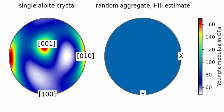
The single-crystal map changes strongly with direction. The aggregate map is constant because the random orientations remove the directional preference.

Read the elastic moduli

Read four familiar moduli from the Voigt tensor. This tensor is the upper bound for the random aggregate.

G = C_iso_Voigt.shearModulus()
G

41.4333

K = C_iso_Voigt.bulkModulus()
K

63.0889

E = C_iso_Voigt.YoungsModulus(xvector)
E

101.9759

nu = C_iso_Voigt.PoissonRatio()
nu

0.2306

The shear modulus \(G\) measures resistance to shape change at fixed volume. The bulk modulus \(K\) measures resistance to a uniform volume change. Young’s modulus \(E\) relates axial stress to axial strain. Poisson’s ratio \(\nu\) is minus transverse strain divided by axial strain.

YoungsModulus asks for a direction. An isotropic tensor gives the same answer in every direction. That equality is a useful check that the average really is isotropic.

E_direction_check = C_iso_Voigt.YoungsModulus(cat(xvector, zvector))
E_direction_check

array([101.9759, 101.9759])

Tighter bounds from a microstructure assumption

The Voigt and Reuss bounds cannot be improved without more information about the material. The microstructures that attain them are extreme: they are layers of aligned crystals.

A quasihomogeneous material has the same elastic properties in any region much larger than a grain. This extra assumption admits narrower bounds. The bounds are due to Hashin and Shtrikman (1962). The computation below follows Brown (2015).

The calculation searches over isotropic comparison materials. Each candidate is specified by a bulk modulus and a shear modulus.

KMin, KMax = 1, 150  # minimum and maximum bulk moduli
GMin, GMax = 1, 150  # minimum and maximum shear moduli
Ko = np.linspace(KMin, KMax, 300)
Go = np.linspace(GMin, GMax, 300)
G0Mesh, K0Mesh = np.meshgrid(Go, Ko)

For every candidate, HashinShtrikmanModulus computes effective bulk and shear moduli. It also tests the residual stiffness tensor. A positive definite residual identifies a lower-bound candidate. A negative definite residual identifies an upper-bound candidate.

khs, ghs, definite = HashinShtrikmanModulus(C, K0Mesh, G0Mesh)

# largest value in the positive definite region: lower bound
khsLower = khs[definite == 1].max()
ghsLower = ghs[definite == 1].max()

# smallest value in the negative definite region: upper bound
khsUpper = khs[definite == -1].min()
ghsUpper = ghs[definite == -1].min()

Locate the Hashin-Shtrikman bounds

Plot the computed effective modulus for every comparison material. The white circles mark the lower and upper optima.

fig, axes = plt.subplots(1, 2, figsize=(10, 5))
for ax, M, lower, upper, name in zip(axes, [khs, ghs], [khsLower, ghsLower], [khsUpper, ghsUpper],
                                     ['effective bulk modulus', 'effective shear modulus']):
  im = ax.imshow(M, extent=[GMin, GMax, KMin, KMax], origin='lower')
  ax.set_title(name)
  ax.set_xlabel('comparison shear modulus')
  ax.set_ylabel('comparison bulk modulus')
  fig.colorbar(im, ax=ax, shrink=0.8)
  for value in (lower, upper):
    i, j = np.nonzero(M == value)
    ax.plot(Go[j], Ko[i], 'o', markeredgecolor='w', markerfacecolor='none', markeredgewidth=2)

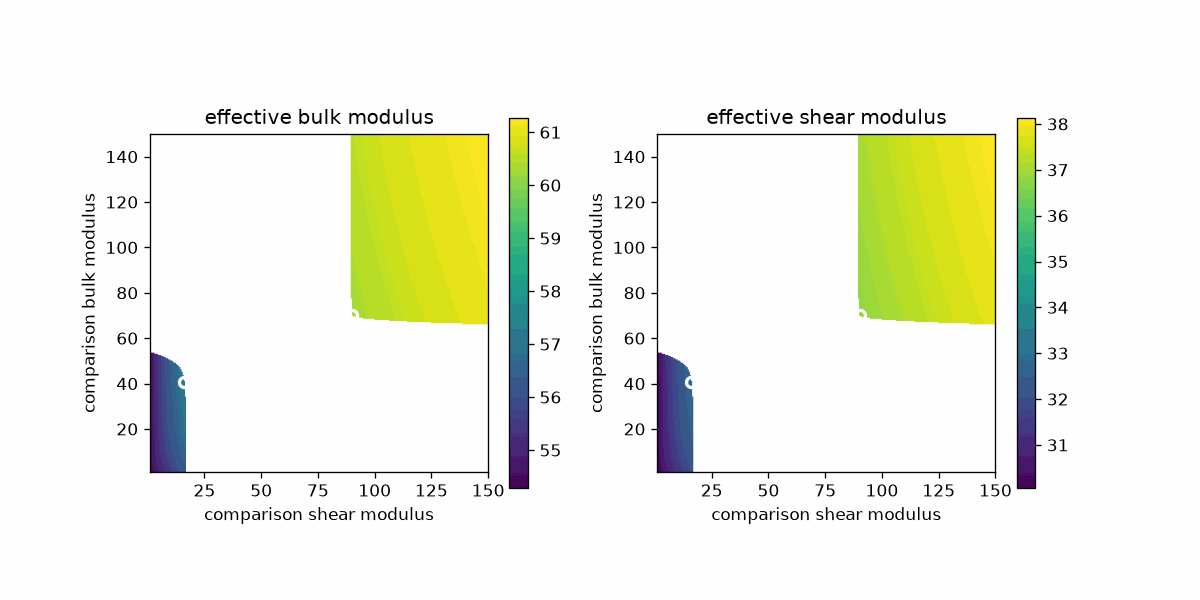
Only the positive and negative definite regions contain valid candidates. The circles sit at the extrema of those two regions, not at arbitrary extrema of the coloured maps.

Compare all three estimates

Collect the Voigt, Reuss, Hill, and Hashin-Shtrikman results.

KReuss = C_iso_Reuss.bulkModulus()
KHill = C_iso_Hill.bulkModulus()
GVoigt = C_iso_Voigt.shearModulus()
GReuss = C_iso_Reuss.shearModulus()
GHill = C_iso_Hill.shearModulus()

print('bulk modulus')
cprintf([K, khsUpper, KHill, khsLower, KReuss], '-Lc', ['Voigt', '+HS', 'Hill', '-HS', 'Reuss'])
print()
print('shear modulus')
cprintf([GVoigt, ghsUpper, GHill, ghsLower, GReuss], '-Lc', ['Voigt', '+HS', 'Hill', '-HS', 'Reuss'])

bulk modulus
  Voigt     +HS    Hill     -HS   Reuss
63.0889  60.326 58.5696  57.107 54.0503

shear modulus
  Voigt     +HS    Hill     -HS   Reuss
41.4333 36.7537 35.6344 32.8495 29.8355

Read the two rows from outside towards the centre. For the bulk modulus, the Voigt and Reuss bounds are 63.1 and 54.1 GPa. They are nine GPa apart. The Hashin-Shtrikman bounds are 60.3 and 57.1 GPa. They are only three GPa apart.

For the shear modulus, the broad interval runs from 41.4 to 29.8 GPa. The Hashin-Shtrikman interval runs from 36.8 to 32.8 GPa. In both rows the Hill average sits inside the narrower pair. This is the reason the Hill estimate usually works.

Bounds on every other modulus follow from these values. Two moduli determine an isotropic material.

The maths behind isotropic stiffness

Any two elastic moduli determine the complete isotropic tensor. Start with the bulk and shear moduli from the Voigt estimate.

C11 = K + (4 / 3) * G
C12 = C11 - 2 * G
C44 = (C11 - C12) / 2

C_from_KG = stiffnessTensor(
  [[C11, C12, C12, 0.0, 0.0, 0.0],
   [C12, C11, C12, 0.0, 0.0, 0.0],
   [C12, C12, C11, 0.0, 0.0, 0.0],
   [0.0, 0.0, 0.0, C44, 0.0, 0.0],
   [0.0, 0.0, 0.0, 0.0, C44, 0.0],
   [0.0, 0.0, 0.0, 0.0, 0.0, C44]], cs)
C_from_KG

stiffnessTensor (An0 Albite 2016)
  unit: GPa
  rank: 4 (3 × 3 × 3 × 3)
  tensor in Voigt matrix representation
  118.3333   35.4667   35.4667        0        0        0
   35.4667  118.3333   35.4667        0        0        0
   35.4667   35.4667  118.3333        0        0        0
         0         0         0  41.4333        0        0
         0         0         0        0  41.4333        0
         0         0         0        0        0  41.4333

Young’s modulus and Poisson’s ratio give the same tensor through its inverse, the compliance tensor.

S11 = 1 / E
S12 = -nu / E
S44 = 2 * (S11 - S12)

C_from_Enu = inv(complianceTensor(
  [[S11, S12, S12, 0.0, 0.0, 0.0],
   [S12, S11, S12, 0.0, 0.0, 0.0],
   [S12, S12, S11, 0.0, 0.0, 0.0],
   [0.0, 0.0, 0.0, S44, 0.0, 0.0],
   [0.0, 0.0, 0.0, 0.0, S44, 0.0],
   [0.0, 0.0, 0.0, 0.0, 0.0, S44]], cs))
C_from_Enu

stiffnessTensor (An0 Albite 2016)
  unit: GPa
  rank: 4 (3 × 3 × 3 × 3)
  tensor in Voigt matrix representation
  118.3333   35.4667   35.4667        0        0        0
   35.4667  118.3333   35.4667        0        0        0
   35.4667   35.4667  118.3333        0        0        0
         0         0         0  41.4333        0        0
         0         0         0        0  41.4333        0
         0         0         0        0        0  41.4333

Both constructions reproduce the averaged tensor above entry for entry. The same equivalence gives direct conversion formulas between moduli.

# two formulas for Poisson's ratio
nu_from_EG = (E / G - 2) / 2
nu_from_KE = (3 * K - E) / (6 * K)

# two formulas for Young's modulus
E_from_Gnu = 2 * G * (1 + nu)
E_from_Knu = 3 * K * (1 - 2 * nu)

np.array([nu_from_EG, nu_from_KE, E_from_Gnu, E_from_Knu])

array([  0.2306,   0.2306, 101.9759, 101.9759])

Lame constants and Hooke’s law

The Lame constants are the pair usually preferred in theoretical work. They make isotropic Hooke’s law especially short.

lam = nu / (1 - 2 * nu) / (1 + nu) * E
mu = G

# rebuild the stiffness tensor from the Lame constants
C_from_Lame = 2 * mu * stiffnessTensor.eye(cs) + lam * dyad(tensor.eye(cs), tensor.eye(cs))
C_from_Lame

stiffnessTensor (An0 Albite 2016)
  unit: GPa
  rank: 4 (3 × 3 × 3 × 3)
  tensor in Voigt matrix representation
  118.3333   35.4667   35.4667        0        0        0
   35.4667  118.3333   35.4667        0        0        0
   35.4667   35.4667  118.3333        0        0        0
         0         0         0  41.4333        0        0
         0         0         0        0  41.4333        0
         0         0         0        0        0  41.4333

Apply Hooke’s law to a random strain, first by tensor contraction.

eps = strainTensor.rand(cs)
sigma_contraction = colon(C_iso_Voigt, eps)
sigma_contraction

stressTensor (y↓→x)
  rank: 2 (3 × 3)
  -77.6652   75.3156  73.4026
   75.3156  -77.8147  -1.7231
   73.4026   -1.7231  -8.9174

The Lame form gives exactly the same stress.

sigma_Lame = stressTensor(2 * mu * eps + lam * trace(eps) * tensor.eye(cs))
sigma_Lame

stressTensor (An0 Albite 2016)
  rank: 2 (3 × 3)
  -77.6652   75.3156  73.4026
   75.3156  -77.8147  -1.7231
   73.4026   -1.7231  -8.9174

References

• J. M. Brown, Determination of Hashin-Shtrikman bounds on the isotropic effective elastic moduli of polycrystals of any symmetry, Computers & Geosciences 80 (2015), 95-99, gives the numerical search used in this page.
• Z. Hashin and S. Shtrikman, A variational approach to the theory of the elastic behaviour of multiphase materials, Journal of the Mechanics and Physics of Solids 11 (1963), 127-140, develops the variational bounds and the quasihomogeneous-material assumption.

Next

Anisotropic Theory removes the directional equality used here. It shows how crystal symmetry constrains a full stiffness tensor and how to read its directional elastic response.

Technical Details

MATLAB’s three outputs of mean(C, odf) are mean(C, odf, 'all') here, the Voigt, Reuss and Hill tensors in that order. The identity tensor.eye(cs) is written in the frame of the crystal, since a tensor without that frame cannot be added to one with it; MATLAB’s tensor.eye borrows the frame of the sum. HashinShtrikmanModulus returns NaN for the comparison materials whose residual is neither positive nor negative definite, which the maps leave white where MATLAB’s imagesc paints them in the lowest colour. The random strain differs from MATLAB’s run, so do the two stresses; they agree with each other.

@article{bachmann2010mtex,
  author  = {F. Bachmann and R. Hielscher and H. Schaeben},
  title   = {Texture Analysis with MTEX - Free and Open Source Software Toolbox},
  journal = {Solid State Phenomena},
  volume  = {160},
  pages   = {63-68},
  year    = {2010},
  doi     = {10.4028/www.scientific.net/SSP.160.63},
  url     = {https://doi.org/10.4028/www.scientific.net/SSP.160.63}
}