Triple-Point-Based Parent Phase Reconstruction

This page reconstructs former beta grains in a titanium alloy from places where three measured alpha grains meet. It continues Grain Graph Based Reconstruction, but uses a triple point rather than a boundary between two grains as its first source of evidence.

import numpy as np

from mtex import *

ebsd = mtexdata('alphaBetaTitanium', verbose=False)

# plot the measured alpha phase with inverse pole figure colours
plot(ebsd['Ti (alpha)'], ebsd['Ti (alpha)'].orientations, figSize='large')

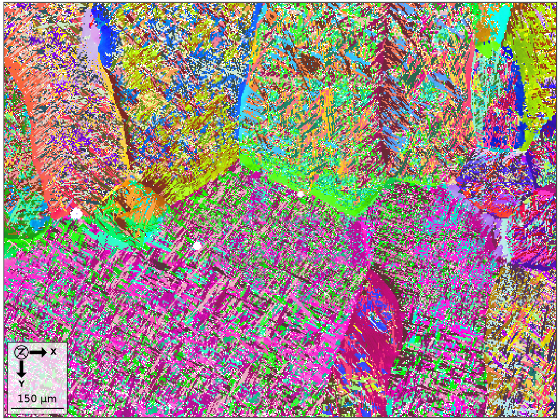
The indexed measurements contain 99.8% alpha titanium and 0.2% beta titanium. The goal is to recover the original beta phase.

phaseFraction = 100 * np.array([len(ebsd['Ti (alpha)']), len(ebsd['Ti (beta)'])]) / len(ebsd['indexed'])
phaseFraction

array([99.7653,  0.2347])

Groups of related alpha colours already suggest the former beta-grain shapes. The reconstruction must turn that visual pattern into a reproducible assignment of parent orientations and boundaries.

Set the parent-to-child orientation relationship

The Burgers orientation relationship (OR) aligns a beta \((110)\) plane with an alpha \((0001)\) plane. It also aligns a beta \([1\bar{1}1]\) direction with an alpha \([\bar{2}110]\) direction.

beta2alpha = orientation.Burgers(ebsd['Ti (beta)'].CS, ebsd['Ti (alpha)'].CS)
beta2alpha

misorientation (Ti (BETA) → Ti (alpha))
  (110) || (0001)   [1̅11̅] || [21̅1̅0]

Parent grain reconstruction functions expect the OR in the parent-to-child direction. Passing the inverse would produce incorrect candidate parent orientations even if the resulting map appeared structured.

Segment the child grains

A grain is a phase-homogeneous, spatially connected region of EBSD pixels produced by segmentation. Triple-point voting needs three separate child grains, so the initial segmentation must not join alpha regions that may have different beta parents.

grains = calcGrains(ebsd, threshold=1.5 * degree, removeQuadruplePoints=True)

The deliberately small 1.5-degree threshold keeps such alpha regions separate. The removeQuadruplePoints option replaces every four-way junction with two three-segment junctions. In this child-phase map, those junctions supply the triple points required by the voting algorithm.

A triple point is a junction where exactly three boundary segments meet and separate three distinct real grains. It therefore provides three child orientations that can be tested against one common parent.

childTriplePoints = grains.triplePoints
childTriplePoints = childTriplePoints[np.all(childTriplePoints.phaseId == grains.cs2phaseId(ebsd['Ti (alpha)'].CS), axis=1)]
numChildTriplePoints = len(childTriplePoints)
print(numChildTriplePoints)

plot(grains.boundary, lineColor=[0.55, 0.55, 0.55], region=[600, 700, 500, 600], figSize='large')
hold(True)
plot(childTriplePoints, color='red', markerSize=5, region=[600, 700, 500, 600])
hold(False)

85338

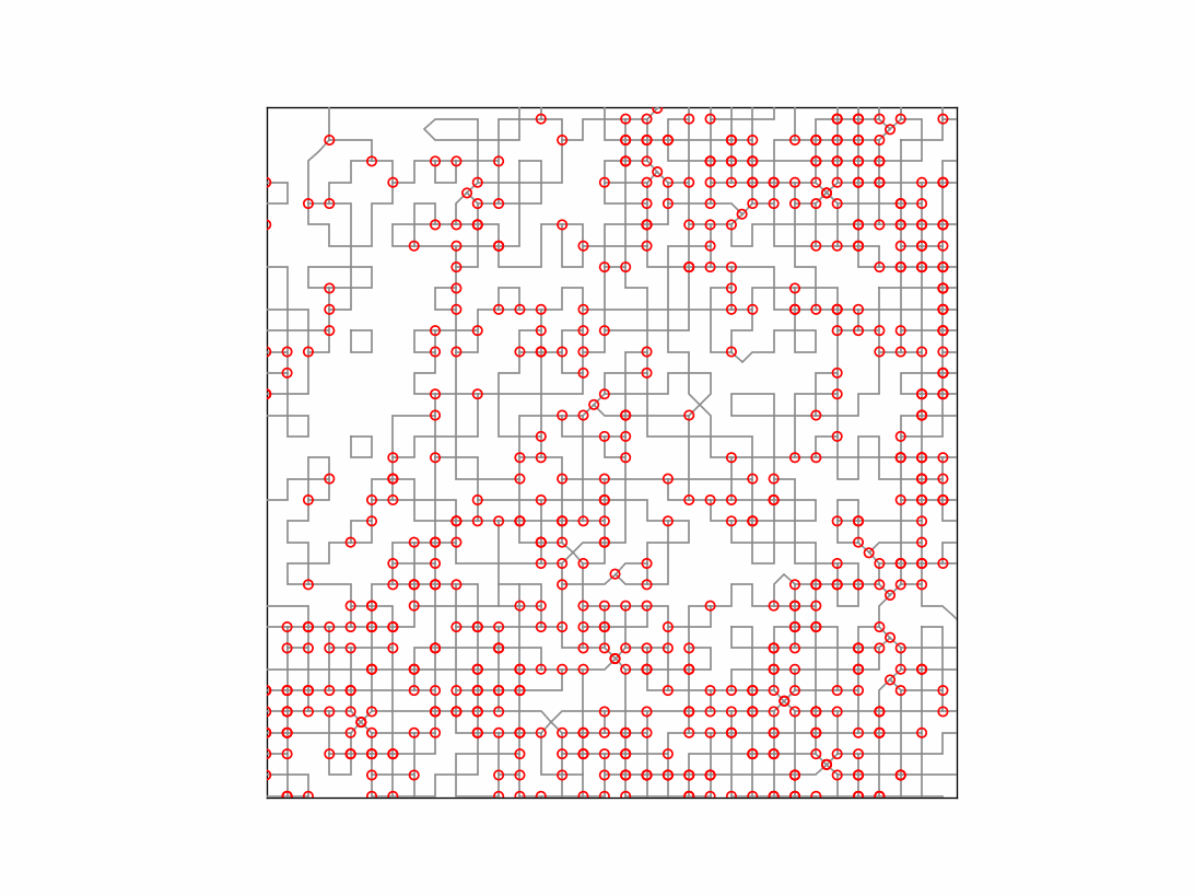
Red markers show the child-child-child triple points used as possible reconstruction seeds. Boundary ends and other junctions are not included.

Set up the reconstruction job

A parentGrainReconstructor stores both the measured child grains and the current reconstruction. Assigning p2c identifies the beta phase as the parent and the alpha phase as the child.

job = parentGrainReconstructor(ebsd, grains)
job.p2c = beta2alpha
job

parentGrainReconstructor

  phase   mineral     symmetry  grains  area   reconstructed
  parent  Ti (BETA)   432       428     0.23%  0%           
  child   Ti (alpha)  622       45804   100%                

 OR: (110) || (0001)   [1̅11̅] || [21̅1̅0]
   p2c fit: 0.82°, 1.2°, 1.6°, 3.1° (quintiles)
   c2c fit: 0.71°, 1°, 1.3°, 1.8° (quintiles)

Find unambiguous triple-point seeds

calcTPVotes asks whether the three child orientations at each triple point are variants of one beta orientation. It computes the best and second-best common-parent fits.

job.calcTPVotes(minFit=2.5 * degree, maxFit=5 * degree)
job

parentGrainReconstructor

  phase   mineral     symmetry  grains  area   reconstructed
  parent  Ti (BETA)   432       428     0.23%  0%           
  child   Ti (alpha)  622       45804   100%                

 OR: (110) || (0001)   [1̅11̅] || [21̅1̅0]
   p2c fit: 0.82°, 1.2°, 1.6°, 3.1° (quintiles)
   c2c fit: 0.71°, 1°, 1.3°, 1.8° (quintiles)

 votes: 37075 × 1
   probabilities: 93%, 88%, 81%, 68% (quintiles)

Despite their option names, the two limits act in opposite directions. minFit requires the best fit to be smaller than 2.5 degrees. maxFit requires the second-best fit to be larger than 5 degrees. A point is therefore retained only when one candidate fits well and its nearest competitor fits distinctly worse. This rejects ambiguous triple points that support two parent orientations almost equally well.

The remaining evidence is accumulated by child grain in job.votes. The first columns of job.votes.parentId and job.votes.prob contain each grain’s highest-ranked parent candidate and its probability.

bestProbability = job.votes.prob[:, 0]
finiteProbability = np.isfinite(bestProbability)
fractionAbove70 = np.count_nonzero(bestProbability[finiteProbability] > 0.7) / np.count_nonzero(finiteProbability)
print(fractionAbove70)

plot(job.grains, bestProbability)
mtexColorbar(title='best vote probability')

0.7799865138233311

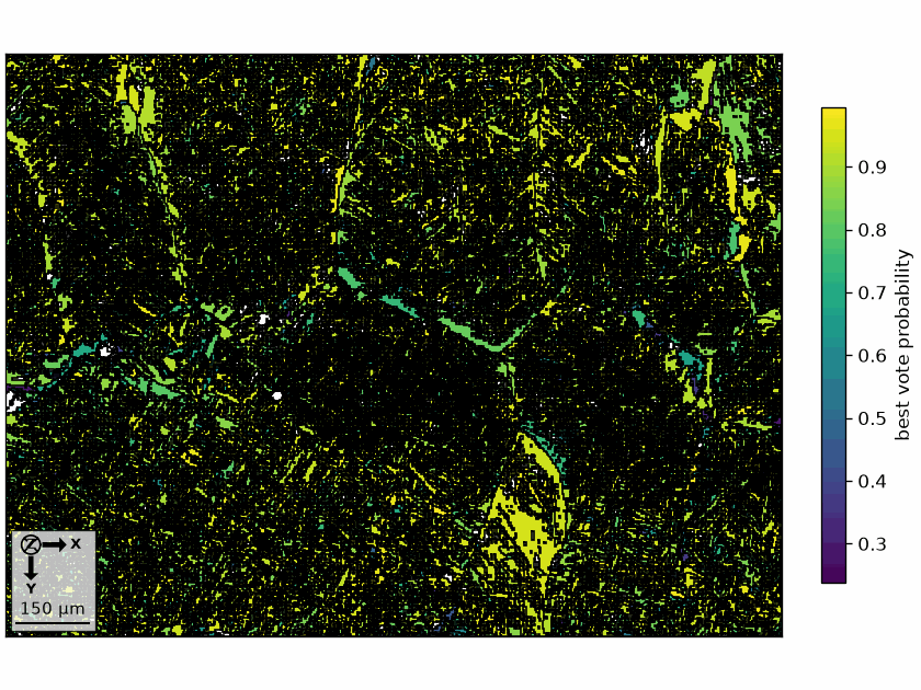
In this run, 77.73% of grains with a finite vote have probability above 70%. The map shows where the accepted triple points provide strong seeds and where no unambiguous three-grain constraint is available.

Transform grains supported by triple-point votes

Transform is the first reconstruction step. Each accepted child grain is assigned its candidate beta orientation and changes from the child phase to the parent phase. It has not yet been merged with neighbouring candidates.

calcParentFromVote applies the 70% probability threshold used above.

job.calcParentFromVote(minProb=0.7)
print(job)

fractionTransformedByTP = np.count_nonzero(job.isTransformed) / np.count_nonzero(job.grainsPrior.phaseId == job.childPhaseId)
fractionTransformedByTP

parentGrainReconstructor

  phase   mineral     symmetry  grains  area  reconstructed
  parent  Ti (BETA)   432       29346   83%   63%          
  child   Ti (alpha)  622       16886   17%                

 OR: (110) || (0001)   [1̅11̅] || [21̅1̅0]
   p2c fit: 0.95°, 1.4°, 1.8°, 2.3° (quintiles)
   c2c fit: 1.1°, 1.6°, 2°, 2.7° (quintiles)

 votes: 8157 × 1
   probabilities: 66%, 60%, 53%, 43% (quintiles)
0.6313

Earlier text reported that more than 66% of the input child grains were transformed by these seeds. The current run gives 62.95%, so that claim no longer holds for the present implementation and data import. The remaining child grains need evidence from reconstructed neighbours.

# define a beta-phase inverse pole figure colour key
ipfKey = ipfColorKey(ebsd['Ti (Beta)'])
ipfKey.ipfDirection = vector3d.Y

# plot the beta candidates produced by the seed step
parentColor = ipfKey.orientation2color(job.parentGrains.meanOrientation)
plot(job.parentGrains, parentColor, figSize='large')

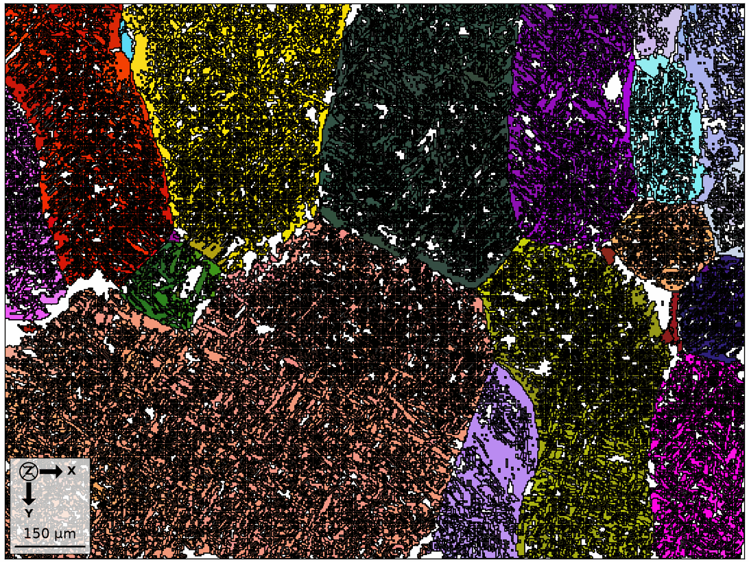
The coloured beta candidates occupy much of the map, but unreconstructed regions remain between them. The next step grows only from parent-child boundaries, so accepted seeds support their immediate child neighbours.

Grow from parent-child boundaries

calcGBVotes with p2c considers only boundaries between a reconstructed parent grain and an unreconstructed child grain. Three passes use thresholds of 2.5, 5, and 7.5 degrees. Newly transformed grains can support the next pass.

childGrainsAfterGrowth = np.zeros(3, dtype=int)
for k in range(1, 4):
  job.calcGBVotes(p2c=True, threshold=k * 2.5 * degree)
  job.calcParentFromVote()
  childGrainsAfterGrowth[k - 1] = len(job.childGrains)

print(childGrainsAfterGrowth)

parentColor = ipfKey.orientation2color(job.parentGrains.meanOrientation)
plot(job.parentGrains, parentColor, figSize='large')

[1612 1125 1098]

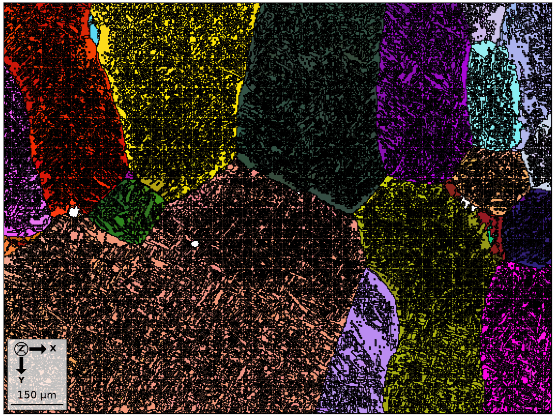
The child-grain counts decrease from 1,609 to 1,127 and then 1,097 as the reconstructed neighbourhood expands. The map fills regions that triple-point votes could not seed while retaining the candidates already accepted.

Merge compatible parent fragments

Merge is the second reconstruction step. It combines neighbouring transformed grains into one parent-grain footprint.

mergeSimilar treats parent neighbours within 5 degrees as parts of the same beta grain.

numParentsBeforeMerge = len(job.parentGrains)
print(numParentsBeforeMerge)
job.mergeSimilar(threshold=5 * degree)
print(job)
numParentsAfterMerge = len(job.parentGrains)
print(numParentsAfterMerge)

parentColor = ipfKey.orientation2color(job.parentGrains.meanOrientation)
plot(job.parentGrains, parentColor, figSize='large')

45134
parentGrainReconstructor

  phase   mineral     symmetry  grains  area   reconstructed
  parent  Ti (BETA)   432       143     99%    98%          
  child   Ti (alpha)  622       1078    0.65%               

 OR: (110) || (0001)   [1̅11̅] || [21̅1̅0]
   p2c fit: 33°, 35°, 41°, 42° (quintiles)
   c2c fit: 6.7°, 17°, 19°, 25° (quintiles)
143

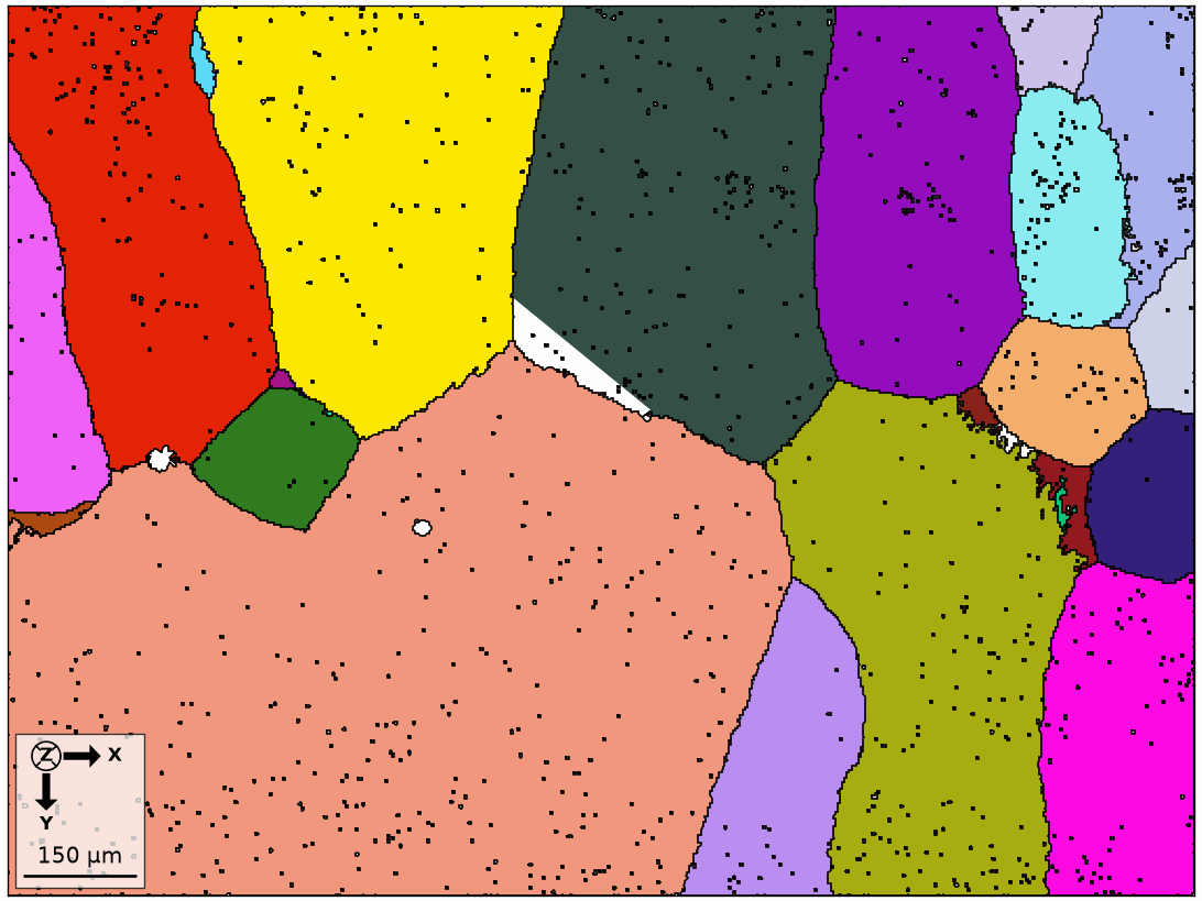
The parent count drops from 45,133 to 144 because similarly oriented fragments now share one footprint. Larger, nearly uniform colour regions replace the fragmented candidates in the preceding map.

Merge small inclusions

An inclusion is a grain entirely enclosed by another grain. Some small child grains remain as inclusions because they never received a sufficiently confident parent orientation.

The earlier description called these poorly indexed inclusions. Here they are unreconstructed indexed child grains; the notIndexed phase is not a reconstruction candidate. mergeInclusions absorbs inclusions of at most five pixels into their surrounding reconstructed parent grains.

numParentsBeforeInclusions = len(job.parentGrains)
print(numParentsBeforeInclusions)
job.mergeInclusions(maxSize=5)
print(job)
numParentsAfterInclusions = len(job.parentGrains)
print(numParentsAfterInclusions)

parentColor = ipfKey.orientation2color(job.parentGrains.meanOrientation)
plot(job.parentGrains, parentColor, figSize='large')

143
parentGrainReconstructor

  phase   mineral     symmetry  grains  area    reconstructed
  parent  Ti (BETA)   432       53      100%    100%         
  child   Ti (alpha)  622       61      0.079%               

 OR: (110) || (0001)   [1̅11̅] || [21̅1̅0]
   p2c fit: 24°, 30°, 33°, 35° (quintiles)
   c2c fit: 6.7°, 13°, 20°, 28° (quintiles)
53

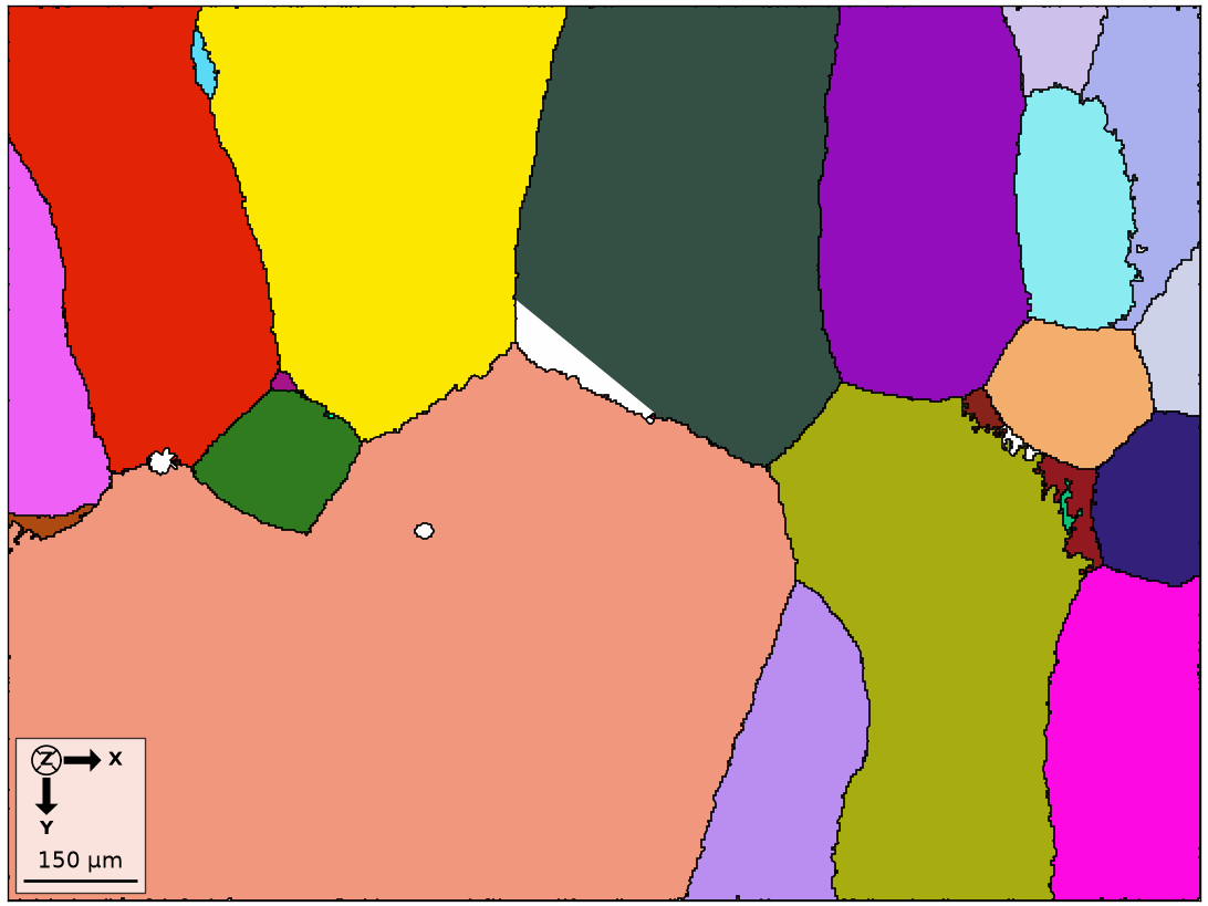
The parent count drops from 144 to 55 as small inclusions are absorbed. The large parent shapes remain, while tiny enclosed child fragments no longer interrupt them. This is a topological cleanup, not a new variant choice.

Reconstruct beta orientations at individual pixels

So far, the reconstructed beta orientations have been stored as grain means. Reading job.ebsd calls calcParentEBSD and returns an EBSD variable with a parent orientation for each transformed child pixel.

parentEBSD = job.ebsd

parentColor = ipfKey.orientation2color(parentEBSD['Ti (Beta)'].orientations)
plot(parentEBSD['Ti (Beta)'], parentColor, figSize='large')

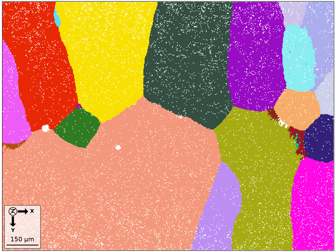
The pixel colours are piecewise consistent with the reconstructed beta grains. The result can now be analysed with ordinary EBSD tools while retaining the reconstructed phase and grain IDs.

Check the per-pixel reconstruction fit

parentEBSD.fit is a per-pixel property. It measures the angular mismatch between a measured alpha orientation and the child variant predicted from its reconstructed beta-grain orientation.

fitDegree = parentEBSD['Ti (Beta)'].fit / degree
fitQuantiles = np.nanquantile(fitDegree[~np.isnan(fitDegree)], [0.5, 0.9, 0.99])
print(fitQuantiles)

plot(parentEBSD, parentEBSD.fit / degree, figSize='large')
mtexColorbar(title='fit (degrees)')
setColorRange([0, 5])
mtexColorMap('LaboTeX')

hold(True)
plot(job.grains.boundary, lineWidth=2)
hold(False)

[1.1886 2.1152 3.777 ]

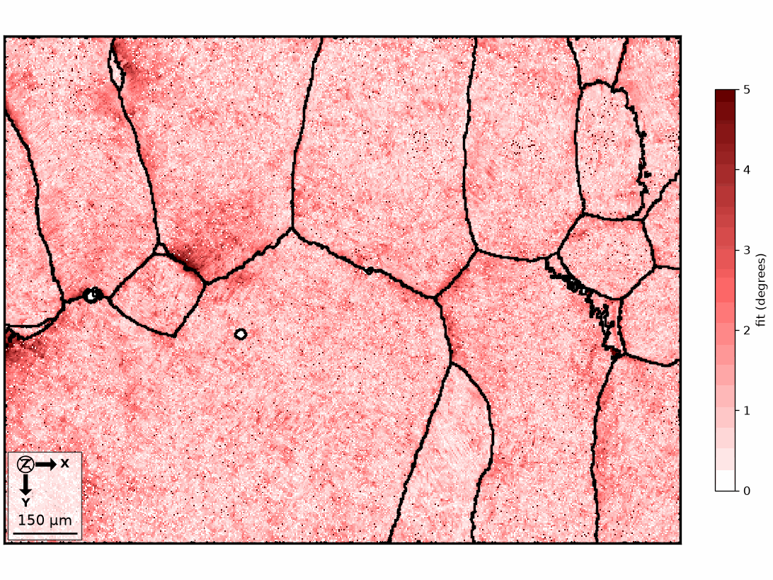
The median fit is 1.189 degrees, 90% are below 2.115 degrees, and 99% are below 3.776 degrees. Low values indicate pixels consistent with their assigned Burgers variant. The black outlines reveal whether larger mismatches collect near reconstructed boundaries.

Compare reconstructed and measured boundaries

The final plot returns to the measured alpha orientations. White lines show the smoothed reconstructed beta-grain boundaries.

plot(ebsd['Ti (Alpha)'], ebsd['Ti (Alpha)'].orientations, figSize='large')

hold(True)
parentGrains = smoothBoundary(job.parentGrains, 5)
plot(parentGrains.boundary, lineWidth=3, lineColor='white')
hold(False)

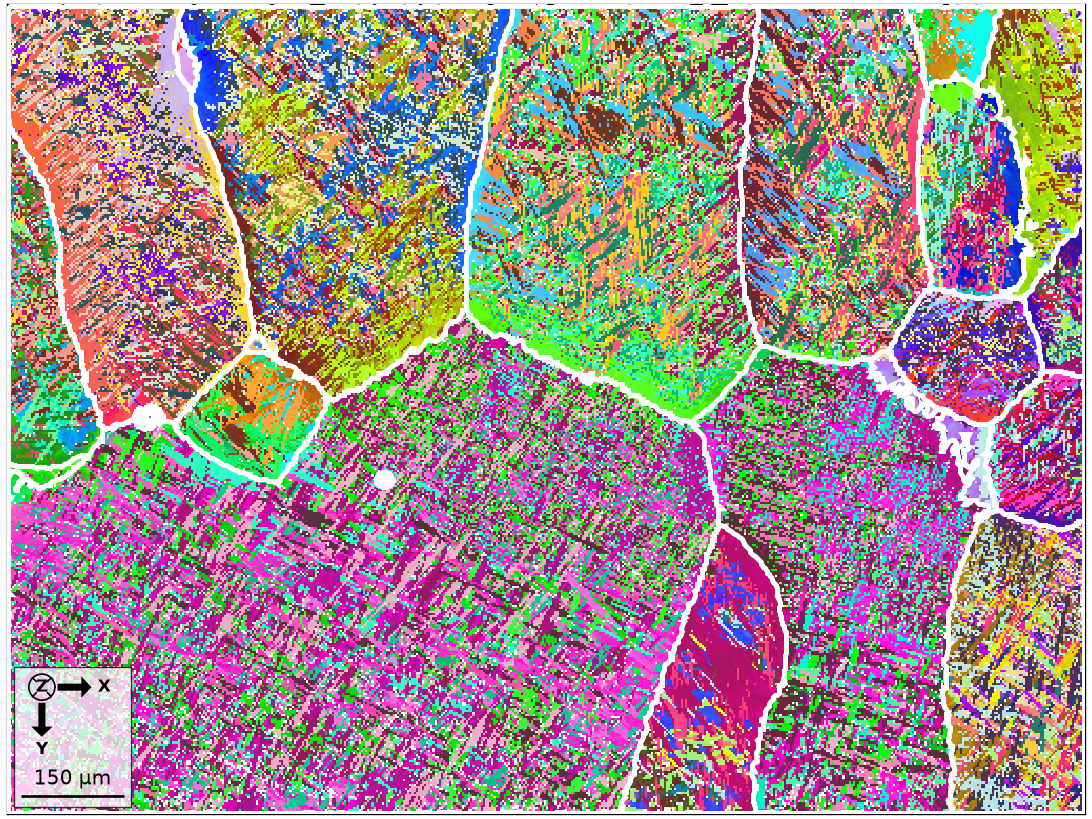
The white outlines enclose groups of alpha orientations that were only suggested by colour in the opening map. This overlay checks whether the reconstructed boundaries follow the visible parent structure.

References

• F. Niessen, T. Nyyssönen, A. A. Gazder, and R. Hielscher, Parent grain reconstruction from partially or fully transformed microstructures in MTEX, Journal of Applied Crystallography 55 (2022), 180-194, defines the generic MTEX reconstruction framework and its triple-point voting strategy.

Next

Continue with Low-Level Parent Grain Reconstruction to compute the same triple-point candidates directly and inspect the fits before assigning parent orientations.

@article{bachmann2010mtex,
  author  = {F. Bachmann and R. Hielscher and H. Schaeben},
  title   = {Texture Analysis with MTEX - Free and Open Source Software Toolbox},
  journal = {Solid State Phenomena},
  volume  = {160},
  pages   = {63-68},
  year    = {2010},
  doi     = {10.4028/www.scientific.net/SSP.160.63},
  url     = {https://doi.org/10.4028/www.scientific.net/SSP.160.63}
}