Grain Graph Based Parent Grain Reconstruction

This page reconstructs prior austenite with a grain graph. It uses the same martensite data as Parent Austenite Reconstruction, but replaces that page’s variant graph with a graph having one node per grain.

The distinction matters. A variant graph decides among candidate variants before merging, while a grain graph reasons directly about compatibility between neighbouring grains. This page concentrates on that second route.

import numpy as np
from scipy.sparse import triu

from mtex import *

plottingConvention.default('y↑→x')
ebsd = mtexdata('martensite', verbose=False)

Segment the child grains

The 3-degree segmentation is deliberately finer than the parent structure. It removes grains below five pixels and smooths the retained boundaries.

grains = calcGrains(ebsd, angle=3 * degree, minPixel=5, alpha=6.1)
grains = smoothBoundary(grains, 5)

plot(ebsd['Iron bcc'], ebsd['Iron bcc'].orientations, figSize='large')
hold(True)
plot(grains.boundary, lineWidth=2)
hold(False)

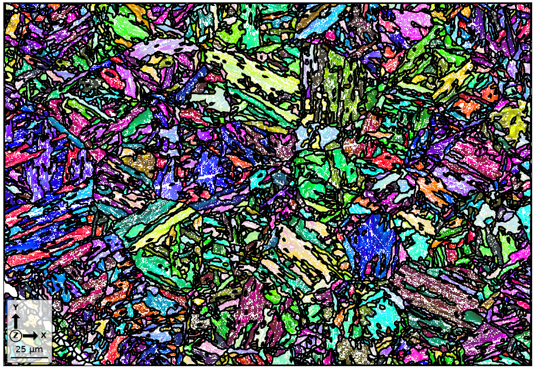
The black child boundaries divide larger groups of related orientation colours. The graph will test which of those boundaries can disappear when the child grains are assigned a common parent.

Set up and fit the orientation relationship

The earlier steel page introduces parentGrainReconstructor and its phase guess. We again start from the Kurdjumov-Sachs (KS) parent-to-child OR. A Nishiyama-Wassermann OR could be supplied as another initial guess.

job = parentGrainReconstructor(ebsd, grains)
initialP2C = orientation.KurdjumovSachs(job.csParent, job.csChild)
job.p2c = initialP2C
print(job)

initialFit = job.calcGBFit()[0] / degree
fitQuantilesInitial = np.nanquantile(initialFit, [0.2, 0.4, 0.6, 0.8])
fitQuantilesInitial

parentGrainReconstructor

  phase   mineral         symmetry  grains  area  reconstructed
  parent  Iron fcc        432       0       0%    0%           
  child   Iron bcc (old)  432       4464    100%               

 OR: (111) || (011)   [101̅] || [111̅]
   c2c fit: 2.4°, 3.4°, 4.4°, 5.5° (quintiles)
array([2.3631, 3.371 , 4.4303, 5.5005])

The former page reported initial fit quintiles of 2.5, 3.5, 4.5, and 5.5 degrees. This run gives 2.363, 3.371, 4.431, and 5.501 degrees. Parent Austenite Reconstruction shows how to overlay the full histograms and map the fit onto boundary segments.

job.calcParent2Child()
print(job)

optimizedFit = job.calcGBFit()[0] / degree
fitQuantilesOptimized = np.nanquantile(optimizedFit, [0.2, 0.4, 0.6, 0.8])
print(fitQuantilesOptimized)
changeFromKS = angle(initialP2C, job.p2c) / degree
changeFromKS

 optimizing parent to child orientation relationship
  scanning 406 orientations
  ( 77.29°,  9.48°,238.25°)  2.824
  ( 77.48°,  9.47°,238.07°)  2.824
parentGrainReconstructor

  phase   mineral         symmetry  grains  area  reconstructed
  parent  Iron fcc        432       0       0%    0%           
  child   Iron bcc (old)  432       4464    100%               

 OR: (77.5°,9.47°,238°)
   c2c fit         : 1.4°, 1.9°, 2.3°, 3.6° (quintiles)
   closest ideal OR: (111) || (201)   [1̅10] || [010] fit: 2.2°
[1.4292 1.8925 2.3094 3.6122]
4.4151

calcParent2Child uses the iterative method of Nyyssönen and co-workers. It assumes that most measured boundaries are child-to-child boundaries. The first fit quintile is 1.453 degrees, consistent with the former rounded value of 1.5 degrees. The change from KS is 3.110 degrees, not 2.3 degrees. The 2.3-degree value in the displayed summary is the distance to the closest rounded ideal OR, so the earlier text compared two different quantities.

Older text said the command stored the misfits in job.fit. The current class has no such property. calcGBFit computes them on demand and also returns their child-grain neighbour pairs. The former reference also paired an unrelated title with a 2018 DOI. The References section gives the OR-fitting paper and DOI used here.

Build the grain graph

A grain graph has one node per grain and one edge per shared grain boundary. An edge weight expresses how compatible the two grains are with a common parent orientation under the fitted OR.

calcGraph derives that weight from the child-to-child misorientation fit. The threshold is the misfit whose weight is exactly one half. The tolerance controls the width of the high-to-low transition. Earlier text called tolerance a Gaussian standard deviation, but the implementation uses it directly as the transition-width parameter.

job.calcGraph(threshold=2.5 * degree, tol=2.5 * degree)
print(job)

graphWeights = triu(job.graph, 1).data
graphWeights = graphWeights[graphWeights != 0]
numGraphEdges = len(graphWeights)
print(numGraphEdges)
graphWeightQuantiles = np.nanquantile(graphWeights, [0.1, 0.5, 0.9])
graphWeightQuantiles

parentGrainReconstructor

  phase   mineral         symmetry  grains  area  reconstructed
  parent  Iron fcc        432       0       0%    0%           
  child   Iron bcc (old)  432       4464    100%               

 OR: (77.5°,9.47°,238°)
   c2c fit         : 1.4°, 1.9°, 2.3°, 3.6° (quintiles)
   closest ideal OR: (111) || (201)   [1̅10] || [010] fit: 2.2°

 graph: 4461 grains in 2 clusters + 4 single grain clusters
11034
array([0.0251, 0.7088, 0.9484])

The printed count is the number of weighted neighbour relations retained by the graph: 11,154 in this run. Its 10th, 50th, and 90th weight percentiles are 0.0080, 0.6677, and 0.9464.

Read the graph on the map

plotGraph maps the edge weights back to their grain boundaries.

plot(ebsd['Iron bcc'], ebsd['Iron bcc'].orientations, figSize='large', faceAlpha=0.5)
hold(True)
job.plotGraph(lineWidth=2)
hold(False)

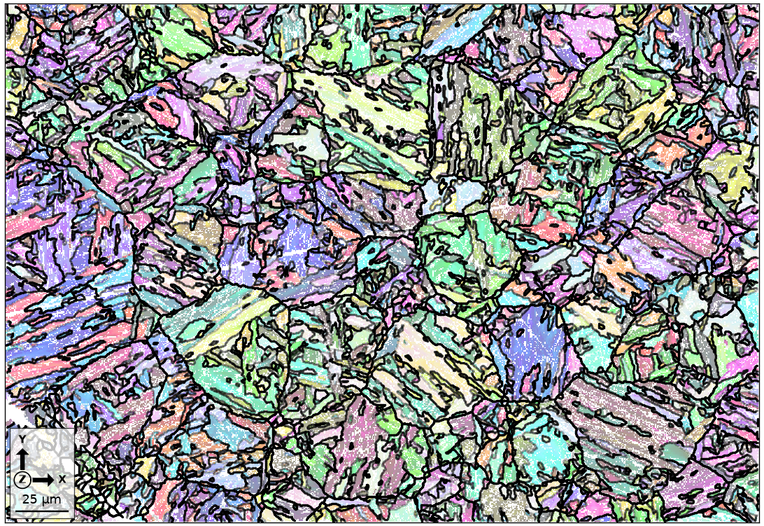
Faint boundaries have high graph weight and are candidates to lie inside one parent grain. Opaque boundaries have weak support and should separate clusters. This inverse transparency is deliberate: likely internal boundaries visually recede.

Cluster the grain graph

clusterGraph uses Markov clustering to turn compatible nodes into components. inflationPower controls their granularity. A smaller value produces fewer, larger clusters; a larger value separates the graph more aggressively.

job.clusterGraph(inflationPower=1.6)
job

parentGrainReconstructor

  phase   mineral         symmetry  grains  area  reconstructed
  parent  Iron fcc        432       0       0%    0%           
  child   Iron bcc (old)  432       4464    100%               

 OR: (77.5°,9.47°,238°)
   c2c fit         : 1.4°, 1.9°, 2.3°, 3.6° (quintiles)
   closest ideal OR: (111) || (201)   [1̅10] || [010] fit: 2.2°

 graph: 4430 grains in 218 clusters + 35 single grain clusters

The displayed graph summary gives clustered grains, component count, and single-grain components. Here 4,414 grains form 237 components and 54 components contain only one grain. These are hypotheses, not yet accepted parent grains.

Transform grains from the graph components

calcParentFromGraph fits one common parent to every component. It then assigns each member its compatible candidate parent orientation. This is the transform step introduced on the earlier steel page. It does not yet merge the component footprints.

job.calcParentFromGraph()
print(job)

numGraphTransformed = np.count_nonzero(job.isTransformed)
print(numGraphTransformed)
plot(job.parentGrains, job.parentGrains.meanOrientation)

parentGrainReconstructor

  phase   mineral         symmetry  grains  area   reconstructed
  parent  Iron fcc        432       4430    100%   99%          
  child   Iron bcc (old)  432       34      0.14%               

 OR: (77.5°,9.47°,238°)
   p2c fit         : 5.4°, 10°, 16°, 24° (quintiles)
   c2c fit         : 3.5°, 3.5°, 3.5°, 3.5° (quintiles)
   closest ideal OR: (111) || (201)   [1̅10] || [010] fit: 2.2°
4430

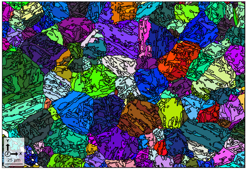
Most child grains now appear in the parent phase. The graph transforms 4,414 grains and leaves 52 child grains unchanged. Neighbouring fragments with similar colours belong to graph components that still await quality control and merging.

Diagnose and reject weak components

job.grains.fit is the angular mismatch between each transformed grain’s candidate parent and the fitted parent of its component. job.grains.clusterSize is the number of grains in that component.

finiteGraphFit = job.grains.fit[np.isfinite(job.grains.fit)] / degree
graphFitQuantiles = np.nanquantile(finiteGraphFit, [0.5, 0.9, 0.99])
print(graphFitQuantiles)

plot(job.grains, job.grains.fit / degree)
setColorRange([0, 5])
mtexColorbar(title='fit (degrees)')

[ 2.0837  4.0717 19.1487]

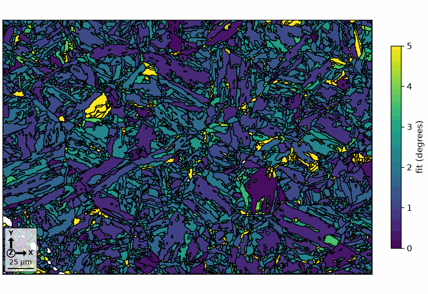
Low values inside a large component support its common parent. High values and isolated small components expose assignments that should be undone before boundary votes use them as neighbours.

rejectGraphAssignment = (job.grains.fit > 5 * degree) | (job.grains.clusterSize < 10)
numGrainsFailingGraphCriteria = np.count_nonzero(rejectGraphAssignment)
print(numGrainsFailingGraphCriteria)

job.revert(rejectGraphAssignment)
print(job)

plot(job.parentGrains, job.parentGrains.meanOrientation)

729
parentGrainReconstructor

  phase   mineral         symmetry  grains  area  reconstructed
  parent  Iron fcc        432       3736    90%   84%          
  child   Iron bcc (old)  432       728     9.5%               

 OR: (77.5°,9.47°,238°)
   p2c fit         : 6.2°, 11°, 15°, 22° (quintiles)
   c2c fit         : 1.4°, 1.8°, 2.2°, 2.9° (quintiles)
   closest ideal OR: (111) || (201)   [1̅10] || [010] fit: 2.2°

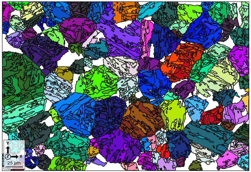
revert restores the measured child phase and orientation for the rejected grains. The criteria flag 848 grains. Of those, 54 carry no graph assignment to undo, so this call reverts 794 of them and leaves 846 child grains. Called without an argument, job.revert() undoes the entire reconstruction. That full reset is useful when comparing graph parameters.

Recover rejected grains with boundary votes

Each boundary to an accepted parent grain votes for a candidate parent of the neighbouring child grain. Three passes let newly transformed grains support the next frontier. Their thresholds relax from 2.5 to 5 and then 7.5 degrees.

childGrainsAfterVote = np.zeros(3, dtype=int)
for k in range(1, 4):
  job.calcGBVotes(p2c=True, threshold=k * 2.5 * degree)
  job.calcParentFromVote()
  childGrainsAfterVote[k - 1] = len(job.childGrains)

print(childGrainsAfterVote)
plot(job.parentGrains, job.parentGrains.meanOrientation)

[554 366 182]

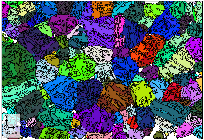
The printed sequence should decrease as the reconstructed neighbourhood expands. It is 614, 387, and 174 child grains in this run. The final map fills most rejected regions without accepting their original weak graph assignments.

Merge parent fragments and inclusions

The earlier steel page defines the separate transform and merge steps. mergeSimilar now combines neighbouring parent fragments within 7.5 degrees. mergeInclusions then absorbs enclosed grains containing at most 50 pixels into their parent host.

numParentsBeforeMerge = len(job.parentGrains)
job.mergeSimilar(threshold=7.5 * degree)
numParentsAfterSimilarMerge = len(job.parentGrains)
job.mergeInclusions(maxSize=50)
numParentsAfterInclusionMerge = len(job.parentGrains)
print(numParentsBeforeMerge, numParentsAfterSimilarMerge, numParentsAfterInclusionMerge)

plot(job.parentGrains, job.parentGrains.meanOrientation)

4282 255 235

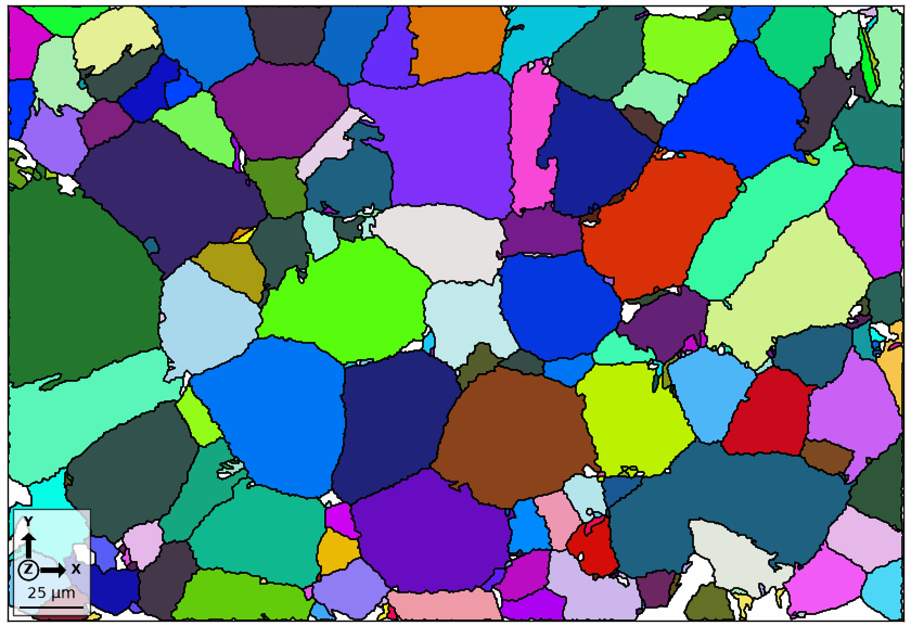
The first count change measures orientation-based merging. The second measures topological inclusion cleanup. Large parent footprints remain while the many compatible fragments and small enclosed child grains disappear.

Check packets and input-to-parent membership

calcVariants stores variantId and packetId on job.transformedGrains. A packet groups variants that share the same parent {111} habit plane. Here packetId selects the parent {111} plane closest to martensite (011).

job.calcVariants()

packetColor = ind2color(job.transformedGrains.packetId - 1)
plot(job.transformedGrains, packetColor, faceAlpha=0.5)

hold(True)
parentGrains = smoothBoundary(job.parentGrains, 10)
plot(parentGrains.boundary, lineWidth=3)
grainSelected = parentGrains[parentGrains.findByLocation([100, 80])]
plot(grainSelected.boundary, lineWidth=3, lineColor='w')
hold(False)

selectedParentId = grainSelected.id
print(selectedParentId)
childGrains = job.grainsPrior[job.mergeId == grainSelected.id]
numChildrenInSelectedParent = len(childGrains)
numChildrenInSelectedParent

[152]
93

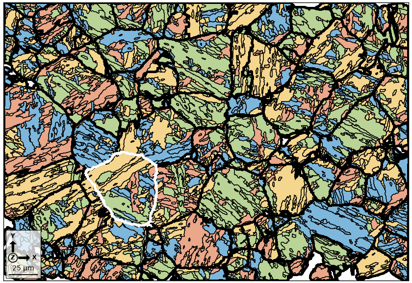
Packet colours should organize inside the thick parent boundaries. The white boundary selects the parent at [100,80]. A parent ID depends on the reconstruction run that produced it, so selectedParentId prints the one this page arrived at rather than a number to carry over from elsewhere.

job.grainsPrior preserves the input grains, while job.mergeId maps each one to its current parent ID. The printed child count confirms the selected footprint can be traced back to its 93 measured grains.

Reuse the common crystallographic and pixel checks

The earlier Parent Austenite Reconstruction works through the remaining checks in full. calcVariantId compares the measured child orientations with all theoretical variants of one reconstructed parent. Its pole figure tests crystallography inside a grain, not only its outline.

calcParentEBSD transfers the grain result to individual pixels. The per-pixel property parentEBSD.fit measures correspondence between the pixel-derived parent and its reconstructed grain orientation.

parentEBSD = job.calcParentEBSD()
pixelFit = parentEBSD['Iron fcc'].fit / degree
pixelFitQuantiles = np.nanquantile(pixelFit, [0.5, 0.9, 0.99])
pixelFitQuantiles

array([2.3266, 4.0804, 7.429 ])

The printed fit quantiles are the compact numerical check for this graph reconstruction. The median, 90th, and 99th percentiles are 2.234, 4.155, and 7.149 degrees. Low values mean the measured child pixels agree with their assigned parent orientation.

To fill remaining notIndexed or not reconstructed pixels, the earlier page segments parentEBSD at 3 degrees with minPixel=10, smooths the parent boundaries by 10 iterations, and applies a halfQuadraticFilter:

parentGrains = calcGrains(parentEBSD, angle=3 * degree, minPixel=10)
parentGrains = smoothBoundary(parentGrains, 10)
F = halfQuadraticFilter()
parentEBSD = smooth(parentEBSD['indexed'], F, fill=parentGrains)

The grain boundaries constrain the fill so it does not blur across the reconstructed parent partition.

Technical Details

On this segmentation the port’s calcParent2Child reaches a lower misfit basin than MATLAB’s (first quintile 1.19 against 1.45 degrees, 3.43 against 3.11 degrees from KS), so every count after the fit differs from the text. With MATLAB’s fitted relationship set as job.p2c the graph route gives MATLAB’s numbers: 11,149 edges with weight percentiles 0.0083, 0.668 and 0.946, 4,411 grains in 236 components with 54 single grains, 839 grains rejected, and 606, 380 and 176 child grains after the three voting passes.

References

• F. Niessen, T. Nyyssönen, A. A. Gazder, and R. Hielscher, Parent grain reconstruction from partially or fully transformed microstructures in MTEX, Journal of Applied Crystallography 55 (2022), 180-194, defines the grain-graph reconstruction, rejection, and boundary-voting workflow used here.
• T. Nyyssönen, M. Isakov, P. Peura, and V.-T. Kuokkala, Iterative determination of the orientation relationship between austenite and martensite from a large amount of grain pair misorientations, Metallurgical and Materials Transactions A 47 (2016), 2587-2590, gives the OR-fitting method.

Next

Continue with Triple Point Based Reconstruction. It replaces pairwise boundary evidence with the stronger constraint available where three distinct grains meet.

@article{bachmann2010mtex,
  author  = {F. Bachmann and R. Hielscher and H. Schaeben},
  title   = {Texture Analysis with MTEX - Free and Open Source Software Toolbox},
  journal = {Solid State Phenomena},
  volume  = {160},
  pages   = {63-68},
  year    = {2010},
  doi     = {10.4028/www.scientific.net/SSP.160.63},
  url     = {https://doi.org/10.4028/www.scientific.net/SSP.160.63}
}